Predicting the perceptual effects of different visual field maps

Every computational model needs to assume a mapping between retinal and visual field coordinates (vfmap). A number of these visual field maps are provided in the topography module:

• Curcio1990Map: The [Curcio1990] model simply assumes that one degree of visual angle (dva) is equal to 280 um on the retina.
• Watson2014Map: The [Watson2014] model extends [Curcio1990] by recognizing that the transformation between dva and retinal eccentricity is not linear (see Eq. A5 in [Watson2014]). However, within 40 degrees of eccentricity, the transform is virtually indistuingishable from [Curcio1990].
• Watson2014DisplaceMap: [Watson2014] also describes the retinal ganglion cell (RGC) density at different retinal eccentricities. In specific, there is a central retinal zone where RGC bodies are displaced centrifugally some distance from the inner segments of the cones to which they are connected through the bipolar cells, and thus from their receptive field (see Eq. 5 [Watson2014]).
• Polimeni2006Map: The [Polimeni2006] model is based on a high-resolution MRI scan of the human visual cortex. It provides a mapping between visual field coordinates and cortical coordinates using a wedge-dipole model for regions V1, V2, and V3. See Appendix B of [Polimeni2006] for details.

• NeuropythyMap: Neuropythy is a python

  package that predicts patient-specific visuotopies based on MRI scans of the human visual cortex. It provides a mapping between visual field coordinates and 3D cortical coordinates for regions V1, V2, V3. See [Benson2018] for details.

All of these visual field maps follow the templates in either RetinalMap or CorticalMap. This means that all retinal visual field maps have to specify a dva_to_ret method, which transforms visual field coordinates into retinal coordinates, and all cortical visual field maps have to specify atleast a dva_to_v1 method, which transforms visual field coordinates into cortical V1 coordinates. Cortical models map also specify dva_to_v2 and dva_to_v3 methods, which transform visual field coordinates into cortical V2 and V3. Most visual field maps also specify the inverse transform, e.g. ret_to_dva or v1_to_dva.

Visual field maps

To appreciate the difference between the available visual field maps, let us look at a rectangular grid in visual field coordinates:

import pulse2percept as p2p
import matplotlib.pyplot as plt

grid = p2p.topography.Grid2D((-50, 50), (-50, 50), step=5)
grid.plot(style='scatter', use_dva=True)
plt.xlabel('x (degrees of visual angle)')
plt.ylabel('y (degrees of visual angle)')
plt.axis('square')

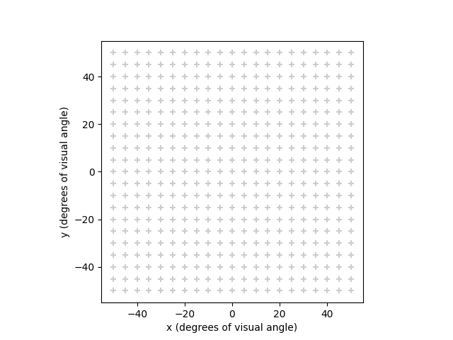
(-55.0, 55.0, -55.0, 55.0)

Such a grid is typically created during a model’s build process and defines at which (x,y) locations the percept is to be evaluated.

However, these visual field coordinates are mapped onto different retinal coordinates under the three visual field maps:

transforms = [p2p.topography.Curcio1990Map(),
              p2p.topography.Watson2014Map(),
              p2p.topography.Watson2014DisplaceMap()]
fig, axes = plt.subplots(ncols=3, sharey=True, figsize=(13, 4))
for ax, transform in zip(axes, transforms):
    grid.build(transform)
    grid.plot(style='cell', ax=ax)
    ax.set_title(transform.__class__.__name__)
    ax.set_xlabel('x (microns)')
    ax.set_ylabel('y (microns)')
    ax.axis('equal')

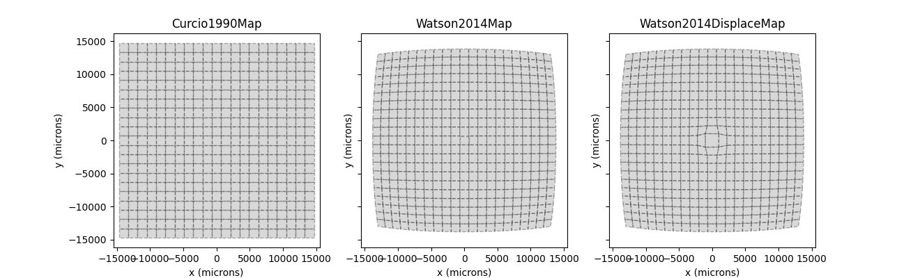
Whereas the [Curcio1990] map applies a simple scaling factor to the visual field coordinates, [Watson2014] uses a nonlinear transform. One thing to note is the RGC displacement zone in the third panel, which might lead to distortions in the fovea.

Perceptual distortions

The perceptual consequences of these visual field maps become apparent when used in combination with an implant.

For this purpose, let us create an AlphaAMS device on the fovea and feed it a suitable stimulus:

implant = p2p.implants.AlphaAMS(stim=p2p.stimuli.LogoUCSB())
implant.stim

Stimulus(data=[[0.], [0.], [0.], ..., [0.], [0.], [0.]],
         dt=0.001,
         electrodes=['A1' 'A2' 'A3' ... 'AN38' 'AN39' 'AN40'],
         is_charge_balanced=False, metadata=dict,
         shape=(1600, 1), time=None)

We can easily switch out the visual field maps by passing a vfmap attribute to ScoreboardModel (by default, the scoreboard model will use [Curcio1990]):

fig, axes = plt.subplots(ncols=3, sharey=True, figsize=(13, 4))
for ax, transform in zip(axes, transforms):
    model = p2p.models.ScoreboardModel(xrange=(-6, 6), yrange=(-6, 6),
                                       vfmap=transform)
    model.build()
    model.predict_percept(implant).plot(ax=ax)
    ax.set_title(transform.__class__.__name__)

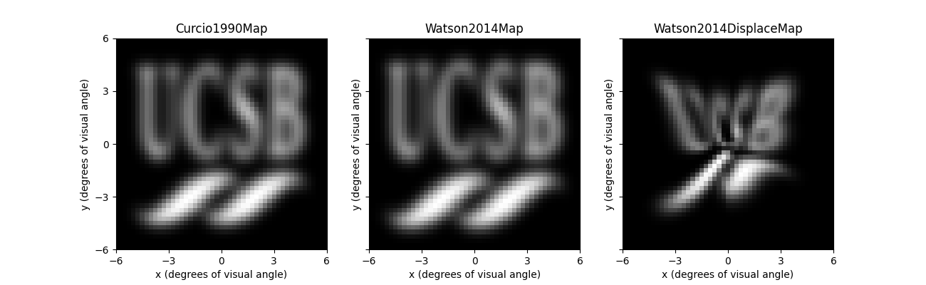
Whereas the left and center panel look virtually identical, the rightmost panel predicts a rather striking perceptual effect of the RGC displacement zone.

Cortical visual field maps

When working with a cortical model (e.g. from pulse2percept.models.cortex), then you should use a cortical visual field map. These maps are subclasses of CorticalMap. Each cortical map has a regions attribute, which specifies the cortical regions that the map uses.

Cortical maps simulate both hemispheres of the visual cortex on a single coordinate plane. The left hemisphere fovea is located at vfmap.left_offset (default: -20 mm), and current is not allowed to spread between hemispheres.

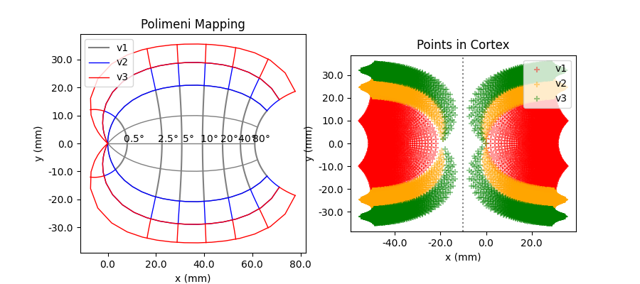
The standard cortical map is Polimeni2006Map, which uses a wedge-dipole model to map visual field coordinates onto cortical coordinates in V1, V2, and V3.

fig, ax = plt.subplots(ncols=2, figsize=(9, 4))
vfmap = p2p.topography.Polimeni2006Map(regions=['v1', 'v2', 'v3']) # simulate all 3 regions
model = p2p.models.cortex.ScoreboardModel(vfmap=vfmap)
model.build()
vfmap.plot(ax=ax[0])
ax[0].set_title('Polimeni Mapping')
model.plot(ax=ax[1])
ax[1].set_title('Points in Cortex')
plt.show()

The Polimeni map has 6 parameters that can be adjusted: k, a global scaling factor; a, and b, which are global wedge-dipole parameters, and alpha1, alpha2, and alpha3, which are azimuthal shear parameters for V1, V2, and V3, respectively. The default values for these parameters are taken from [Polimeni2006] based on MRI fits to human visual cortex. These values are known to change dramatically between individuals, so it may be important to adjust these parameters to fit the individual subject.

Creating your own visual field map

To create your own (retinal) visual field map, you need to subclass the RetinalMap template and provide your own dva_to_ret and ret_to_dva methods. For example, the following class would (wrongly) assume that retinal coordinates are identical to visual field coordinates:

class MyVisualFieldMap(p2p.topography.RetinalMap):

    def dva_to_ret(self, xdva, ydva):
        return xdva, ydva

    def ret_to_dva(self, xret, yret):
        return xret, yret

To use it with a model, you need to pass vfmap=MyVisualFieldMap() to the model’s constructor.