Note
Go to the end to download the full example code.
Horsager et al. (2009): Predicting temporal sensitivity
This example shows how to use the
Horsager2009Model.
The model introduced in [Horsager2009] assumes that electrical stimulation leads to percepts that quickly increase in brightness (over the time course of ~100ms) and then slowly fade away (over the time course of seconds).
The model was fit to perceptual sensitivity data for a number of different
pulse trains, which are available in the datasets
subpackage.
The dataset can be loaded as follows:
from pulse2percept.datasets import load_horsager2009
data = load_horsager2009()
data.shape
(608, 21)
Single-pulse thresholds
Loading the data
The data includes a number of thresholds measured on single-pulse stimuli. We can load a subset of these data; for example, for subject S05 and Electrode C3:
single_pulse = load_horsager2009(subjects='S05', electrodes='C3',
                                 stim_types='single_pulse')
single_pulse
Creating the stimulus
To recreate Fig. 3 in the paper, where the model fit to single-pulse stimuli is shown, we first need to recreate the stimulus used in the figure.
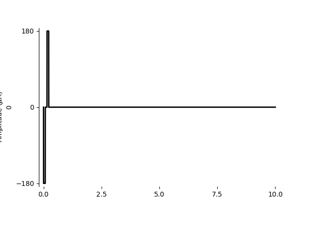
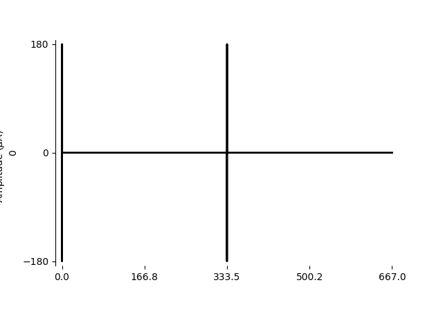
For example, we can create a stimulus from a single biphasic pulse (0.075 ms phase duration) with amplitude 180 uA, lasting 200 ms in total:
import numpy as np
from pulse2percept.stimuli import BiphasicPulse
phase_dur = 0.075
stim_dur = 200
pulse = BiphasicPulse(180, phase_dur, interphase_dur=phase_dur,
                      stim_dur=stim_dur, cathodic_first=True)
pulse.plot(time=np.linspace(0, 10, num=10000))
<Axes: ylabel='0'>
Simulating the model response
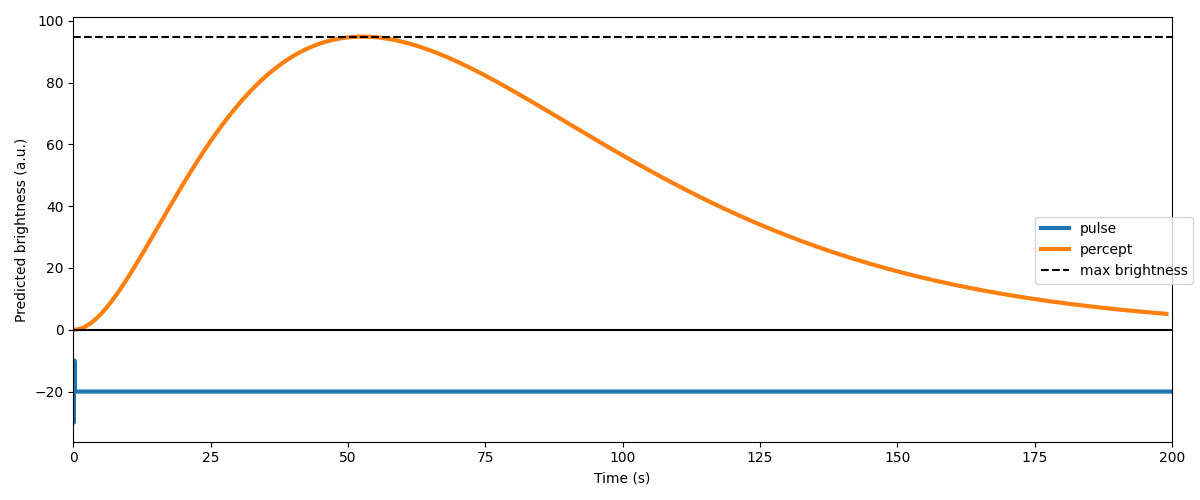
The model’s response to this stimulus can be visualized as follows:
from pulse2percept.models import Horsager2009Temporal
model = Horsager2009Temporal()
model.build()

percept = model.predict_percept(pulse, t_percept=np.arange(stim_dur))

max_bright = percept.data.max()

import matplotlib.pyplot as plt
fig, ax = plt.subplots(figsize=(12, 5))
ax.plot(pulse.time, -20 + 10 * pulse.data[0, :] / pulse.data.max(),
        linewidth=3, label='pulse')
ax.plot(percept.time, percept.data[0, 0, :], linewidth=3, label='percept')
ax.plot([0, stim_dur], [max_bright, max_bright], 'k--', label='max brightness')
ax.plot([0, stim_dur], [0, 0], 'k')

ax.set_xlabel('Time (s)')
ax.set_ylabel('Predicted brightness (a.u.)')
ax.set_xlim(0, stim_dur)
fig.legend(loc='center right')
fig.tight_layout()
Finding the threshold current
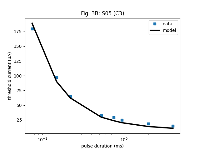
Finally, we need to find the “threshold current” to ultimately reproduce Fig. 3. In the real world, the threshold current is defined as the stimulus amplitude needed to elicit a detectable phosphene (e.g.) 50% of the time. This threshold current typically differs for every stimulus, stimulated electrode, and patient.
In the model, there is no notion of “seeing something 50% of the time”. Instead, the model was assumed to reach threshold if the model response exceeded some constant \(\\theta\) over time.
The process of finding the stimulus amplitude needed to achieve model output
\(\\theta\) can be automated with the help of the
find_threshold() method.
We will run this method on every data point from the ones selected above:
amp_th = []
for _, row in single_pulse.iterrows():
        # Set up a biphasic pulse with amplitude 1uA - the amplitude will be
        # up-and-down regulated by find_threshold until the output matches
        # theta:
    stim = BiphasicPulse(1, row['pulse_dur'],
                         interphase_dur=row['interphase_dur'],
                         stim_dur=row['stim_dur'],
                         cathodic_first=True)
    # Find the current that gives model output theta. Search amplitudes in the
    # range [0, 300] uA. Stop the search once the candidate amplitudes are
    # within 1 uA, or the model output is within 0.1 of theta:
    amp_th.append(model.find_threshold(stim, row['theta'],
                                       amp_range=(0, 300), amp_tol=1,
                                       bright_tol=0.1))

plt.semilogx(single_pulse.pulse_dur, single_pulse.stim_amp, 's', label='data')
plt.semilogx(single_pulse.pulse_dur, amp_th, 'k-', linewidth=3, label='model')
plt.xticks([0.1, 1, 4])
plt.xlabel('pulse duration (ms)')
plt.ylabel('threshold current (uA)')
plt.legend()
plt.title('Fig. 3B: S05 (C3)')
Text(0.5, 1.0, 'Fig. 3B: S05 (C3)')
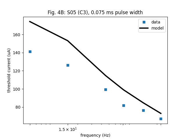
Fixed-duration pulse train thresholds
The same procedure can be repeated for
BiphasicPulseTrain stimuli to reproduce
Fig. 4.
from pulse2percept.stimuli import BiphasicPulseTrain

# Load the data:
fixed_dur = data[(data.stim_type == 'fixed_duration') &
                 (data.subject == 'S05') &
                 (data.electrode == 'C3') &
                 (data.pulse_dur == 0.075)]

# Find the threshold:
amp_th = []
for _, row in fixed_dur.iterrows():
    stim = BiphasicPulseTrain(row['stim_freq'], 1, row['pulse_dur'],
                              interphase_dur=row['interphase_dur'],
                              stim_dur=row['stim_dur'], cathodic_first=True)
    amp_th.append(model.find_threshold(stim, row['theta'],
                                       amp_range=(0, 300), amp_tol=1,
                                       bright_tol=0.1))

plt.semilogx(fixed_dur.stim_freq, fixed_dur.stim_amp, 's', label='data')
plt.semilogx(fixed_dur.stim_freq, amp_th, 'k-', linewidth=3, label='model')
plt.xticks([5, 15, 75, 225])
plt.xlabel('frequency (Hz)')
plt.ylabel('threshold current (uA)')
plt.legend()
plt.title('Fig. 4B: S05 (C3), 0.075 ms pulse width')
Text(0.5, 1.0, 'Fig. 4B: S05 (C3), 0.075 ms pulse width')
Other stimuli
Bursting pulse triplets
“Bursting pulse triplets” as shown in Fig. 7 are readily supported via the
BiphasicTripletTrain class.
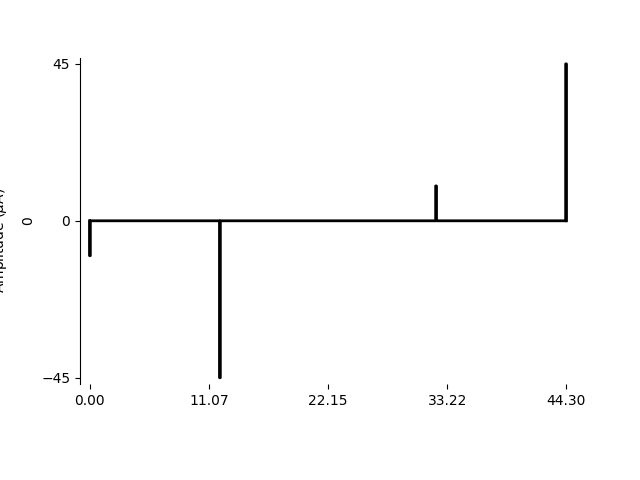
Variable-duration pulse trains
A “variable-duration” pulse train is essentially
BiphasicPulseTrain cut to the length of
N pulses.
For example, the following recreates a pulse train used in Fig. 5B:
<Axes: ylabel='0'>
Latent addition
“Latent addition” stimuli only show up in the supplementary materials (see Fig. S2.2).
They are pseudo-monophasic pulse pairs, where the anodic phases were presented 20 ms after the end of the second cathodic pulse.
The initial cathodic pulse always has a fixed amplitude of 50% of the single pulse threshold:
from pulse2percept.stimuli import MonophasicPulse

# Phase duration:
phase_dur = 0.075

# Single-pulse threshold determines this current:
amp_th = 20

# Cathodic phase of the standard pulse::
cath_stand = MonophasicPulse(-0.5 * amp_th, phase_dur)
The delay between the start of the conditioning pulse and the start of the test pulse was varied systematically (between 0.15 and 12 ms). The amplitude of the second pulse was varied to determine thresholds.
The anodic phase were always presented 20 ms after the second cathodic phase:
anod_stand = MonophasicPulse(0.5 * amp_th, phase_dur, delay_dur=20)

anod_test = MonophasicPulse(amp_test, phase_dur, delay_dur=delay_dur)
The last step is to concatenate all the pulses into a single stimulus:
from pulse2percept.stimuli import Stimulus

latent_add = cath_stand.append(cath_test).append(anod_stand).append(anod_test)
latent_add.plot()
<Axes: ylabel='0'>
Total running time of the script: (0 minutes 0.445 seconds)