Granley et al. (2021): Effects of Biphasic Pulse Parameters with the BiphasicAxonMapModel

This example shows how to use the BiphasicAxonMapModel to model the effects of biphasic pulse train parameters phosphene appearance in an epiretinal implant such as ArgusII.

Biphasic pulse trains are a commonly used type of stimulus in visual prostheses. This model enhances the AxonMapModel to reflect the effects of the amplitude, frequency, and pulse duration on threshold, phosphene size, brightness, and streak length, according to previous psychophysical and electrophysiological studies.

The BiphasicAxonMapModel shares the same underlying assumptions as the axon map model. Namely, an axon’s sensitivity to electrical stimulation is assumed to decay exponentially with…

• distance along the axon from the soma (\(d_s\)), with spatial decay constant \(\lambda\),
• distance from the stimulated electrode (\(d_e\)), with spatial decay constant \(\rho\).

In the biphasic model, the radial decay rate \(\rho\) is scaled by \(F_{size}\), the axonal decay rate \(\lambda\) is scaled by \(F_{streak}\), and the brightness contribution from each electrode is scaled by \(F_{bright}\). These 3 equations are called effect models. The final equation for the brightness intensity for a pixel located at polar coordinates \((r, \theta)\) is given by:

\[I = \max_{axon}\sum_{elecs}F_\mathrm{bright} \exp\left(\frac{-d_{e}^2}{2\rho^2 F_\mathrm{size} } + \frac{-d_{s}^2}{2\lambda^2 F_\mathrm{streak} }\right).\]

Basic Model Usage

The biphasic axon map model can be instantiated and ran similarly to other models, with the exception that all stimuli are required to be BiphasicPulseTrain

import matplotlib.pyplot as plt
import numpy as np
from pulse2percept.implants import ArgusII
from pulse2percept.models import BiphasicAxonMapModel
from pulse2percept.stimuli import BiphasicPulseTrain
model = BiphasicAxonMapModel(rho=200, axlambda=800)

Parameters you don’t specify will take on default values. You can inspect all current model parameters as follows:

print(model)

BiphasicAxonMapModel(ax_segments_range=(0, 50),
                     axlambda=800,
                     axon_pickle='axons.pickle',
                     axons_range=(-180, 180),
                     bright_model=DefaultBrightModel,
                     engine=None, eye='RE',
                     grid_type='rectangular',
                     ignore_pickle=False,
                     loc_od=(15.5, 1.5),
                     min_ax_sensitivity=0.001,
                     n_ax_segments=500, n_axons=1000,
                     n_gray=None, n_jobs=1, n_threads=2,
                     noise=None, retinotopy=Watson2014Map,
                     rho=200, scheduler='threading',
                     size_model=DefaultSizeModel,
                     spatial=BiphasicAxonMapSpatial,
                     streak_model=DefaultStreakModel,
                     temporal=None, thresh_percept=0,
                     verbose=True, xrange=(-15, 15),
                     xystep=0.25, yrange=(-15, 15))

The most important parameters are rho and axlambda, which control the radial and axonal current spread, respectively. The parameters a0-a9 are coefficients for the size, streak, and bright models, which will be discussed later in this example. The biphasic axon map model supports both the default cython engine and a faster, gpu-enabled jax engine.

The rest of the parameters are shared with AxonMapModel. For full details on these parameters, see the Axon Map Tutorial

Next, build the model to perform expensive, one time calculations, and specify a visual prosthesis from the implants module. Models with an axon map are well suited for epiretinal implants, such as Argus II.

model.build()
implant = ArgusII()

Important

You need to build a model only once. After that, you can apply any number of stimuli – or even apply the model to different implants – without having to rebuild (which takes time).

However, if you change model parameters (e.g., by directly setting model.a5 = 2), you will have to call model.build() again for your changes to take effect.

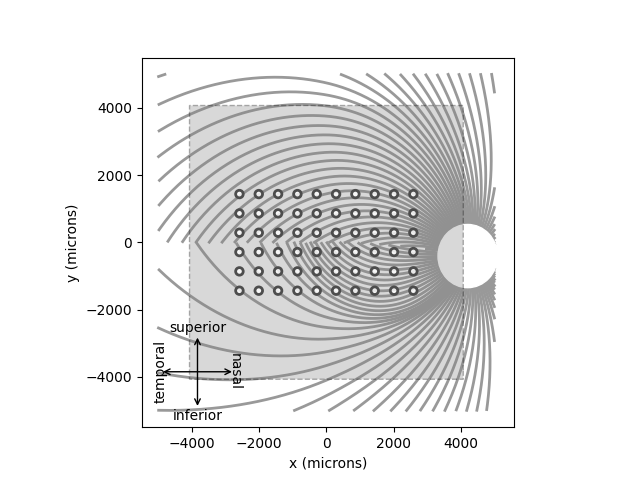
You can visualize the location of the implant and the axon map

model.plot()
implant.plot()
plt.show()

As mentioned above, the Biphasic Axon Map Model only accepts BiphasicPulseTrain stimuli with no delay_dur. The amplitude given to the BiphasicPulseTrain is interpreted as amplitude as a factor of threshold (i.e. an amp of 1 means 1xTh)

You can easily assign BiphasicPulseTrains to electrodes with a dictionary The following creates a train with 20Hz frequency, 1xTh amplitude, and 0.45ms pulse / phase duration.

implant.stim = {'A4' : BiphasicPulseTrain(20, 1, 0.45)}
implant.stim.plot()

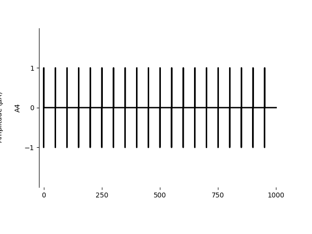
<AxesSubplot:ylabel='A4'>

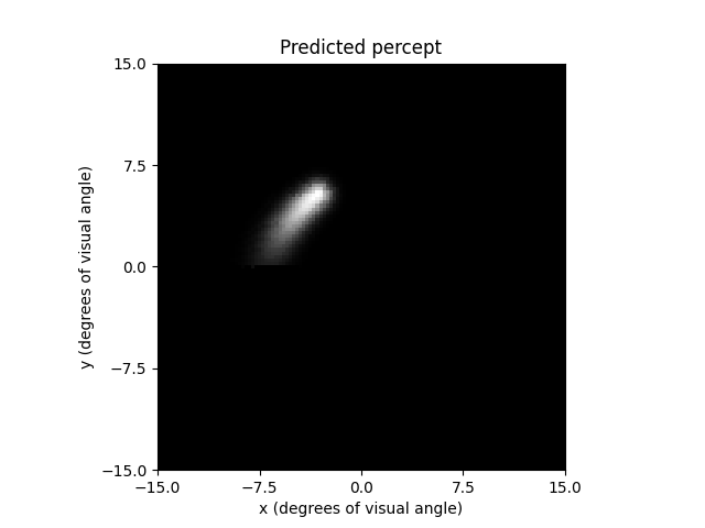
Finally, you can predict the percept resulting from stimulation

percept = model.predict_percept(implant)
ax = percept.plot()
ax.set_title('Predicted percept')
plt.show()

Increasing the frequency will make phosphenes brighter

fig, axes = plt.subplots(1, 2, sharex=True, sharey=True)
implant.stim = {'A4' : BiphasicPulseTrain(50, 1, 0.45)}
new_percept = model.predict_percept(implant)
new_percept.plot(ax=axes[1])
percept.plot(ax=axes[0], vmax=new_percept.max())
axes[0].set_title("20 Hz")
axes[1].set_title("40 Hz")
plt.show()

Note that without setting vmax, matplotlib automatically rescales images to have the same max brightness and the difference isn’t visible

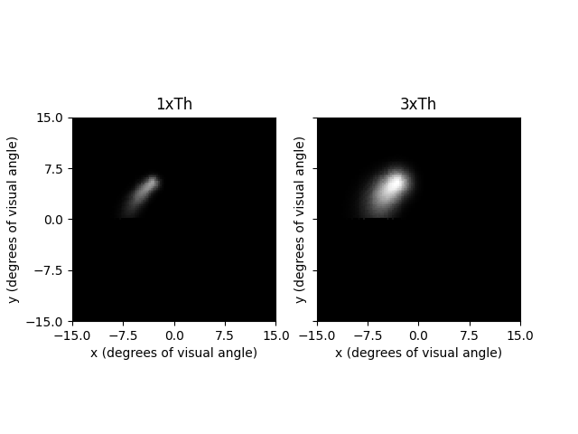
Increasing amplitude increases both size and brightness

fig, axes = plt.subplots(1, 2, sharex=True, sharey=True)
implant.stim = {'A4' : BiphasicPulseTrain(20, 3, 0.45)}
new_percept = model.predict_percept(implant)
new_percept.plot(ax=axes[1])
percept.plot(ax=axes[0], vmax=new_percept.max())
axes[0].set_title("1xTh")
axes[1].set_title("3xTh")
plt.show()

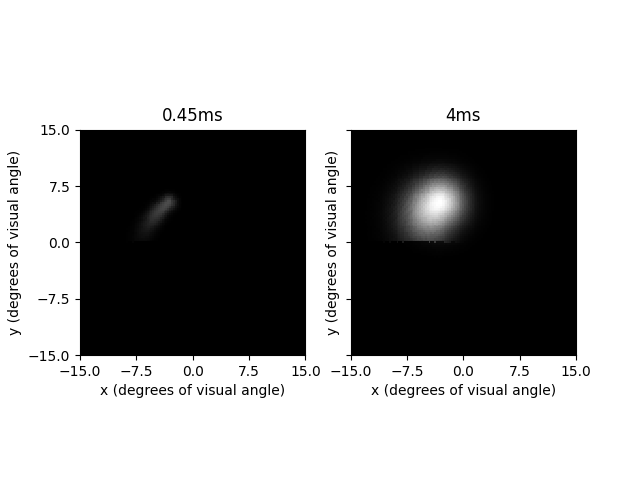
Increasing pulse duration decreases threshold, thus indirectly causing an increase in size and brightness (amp factor is increased)

fig, axes = plt.subplots(1, 2, sharex=True, sharey=True)
implant.stim = {'A4' : BiphasicPulseTrain(20, 1, 4)}
new_percept = model.predict_percept(implant)
new_percept.plot(ax=axes[1])
percept.plot(ax=axes[0], vmax=new_percept.max())
axes[0].set_title("0.45ms")
axes[1].set_title("4ms")
plt.show()

If you account for the change in threshold by decreasing amplitude, then the only affect of increasing pulse duration is the streak length decreasing

fig, axes = plt.subplots(1, 2, sharex=True, sharey=True)
implant.stim = {'A4' : BiphasicPulseTrain(20, 0.023835, 20)}
new_percept = model.predict_percept(implant)
new_percept.plot(ax=axes[1])
percept.plot(ax=axes[0], vmax=new_percept.max())
axes[0].set_title("0.45ms")
axes[1].set_title("20ms, 0.02xTh")
plt.show()

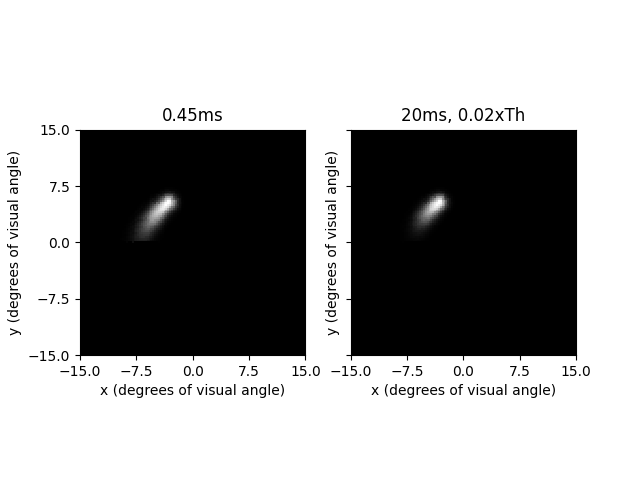
This illustrates another important point: The amplitude used for the Biphasic model is relative to the threshold current at 0.45ms pulse duration. Since larger pulse durations have been shown to reduce the threshold amplitude needed, the 0.02xTh amplitude used in the previous plot still is able to produce a phosphene.

Changing Effect Models

All of the ‘effects’ plotted above (e.g. size increasing with amplitude) are controlled by the effect models \(F_{bright}\), \(F_{size}\), and \(F_{streak}\). The variables bright_model, size_model, and streak_model encode the effects models.

These default to DefaultBrightModel, DefaultSizeModel, and DefaultStreakModel respectively, which implement the simple scaling functions described in Granley et al. (2021).

The coefficients a0-a9 parametrize these effect models. While the default values are likely to work for most cases, they can be customized to be patient specific. Notice how we only have to change the value given to the BiphasicAxonMapModel, and it is automatically passed down to the effect models.

model.a5 = 0
print(model.size_model.a5)

0

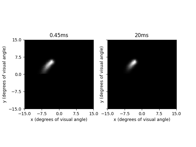
For example, a0 and a1 control how threshold changed with pulse duration: \(amp = (A_0*pdur + A_1)^{-1}*amp\). Thus, pulse duration threshold scaling can easily be disabled by setting a0 to 0 and a1 to 1. If we increase pulse duration like we did previously, we will now see that only streak length decreases, and we no longer have to change amplitude to account for change in threshold

model = BiphasicAxonMapModel(rho=200, axlambda=800)
model.a0 = 0
model.a1 = 1
model.build()
fig, axes = plt.subplots(1, 2, sharex=True, sharey=True)
implant.stim = {'A4' : BiphasicPulseTrain(20, 1, 0.45)}
percept = model.predict_percept(implant)
implant.stim = {'A4' : BiphasicPulseTrain(20, 1, 20)}
new_percept = model.predict_percept(implant)
new_percept.plot(ax=axes[1])
percept.plot(ax=axes[0], vmax=new_percept.max())
axes[0].set_title("0.45ms")
axes[1].set_title("20ms")
plt.show()

Similarly, a2-a4 control brightness scaling; a5-a6 control size scaling, and a7-a9 control streak length scaling. For more details on these parameters, see the effect models documentation, or [Granley2021]

Advanced Usage

Custom Effect Models

For most cases, using the provided, default implementation of the effect models will probably be enough. However, the effect models are completely modular, and can be replaced by any python callable with the parameters frequency, amplitude, and pulse duration. For example, we can easily change the model to no longer scale size

model = BiphasicAxonMapModel(rho=200, axlambda=800)
def size_modulation(freq, amp, pdur):
    return 1
model.size_model = size_modulation
model.build()

fig, axes = plt.subplots(1, 2, sharex=True, sharey=True)
implant.stim = {'A4' : BiphasicPulseTrain(20, 1, 0.45)}
percept = model.predict_percept(implant)
implant.stim = {'A4' : BiphasicPulseTrain(20, 3, 0.45)}
new_percept = model.predict_percept(implant)
new_percept.plot(ax=axes[1])
percept.plot(ax=axes[0], vmax=new_percept.max())
axes[0].set_title("1xTh")
axes[1].set_title("3xTh")
plt.show()

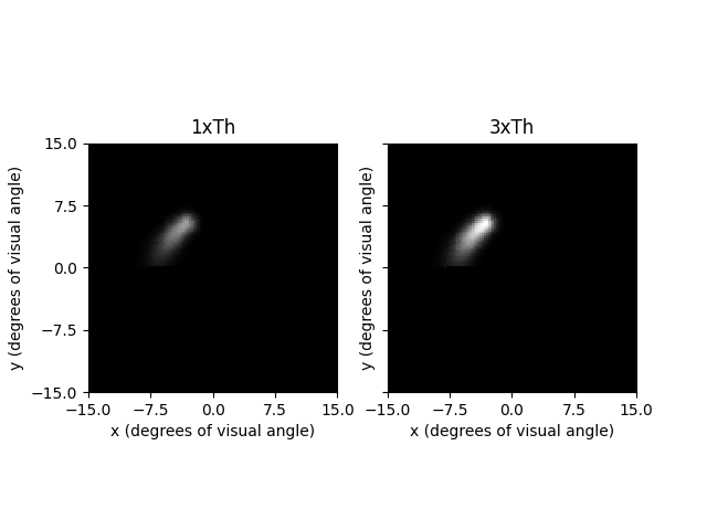
The stimuli with larger amplitude created a brighter, but equally-sized phosphene

The effect models can even be a class, and can have its own parameters, which can be shared with the overarching BiphasicAxonMapModel itself (e.g. an effect model can depend on rho, and if model.rho is changed, rho will also be changed in the effect model). For an example of this, see DefaultSizeModel

If using custom effect models with jax, the effect models must be written for jax so they can be JIT compiled (i.e. using jax.numpy instead of numpy)

JAX Engine

The default computational engine is cython, but an engine based on jax is also provided. The jax engine is slightly faster on CPU and significantly faster on GPU, at the cost of increased memory usage. The jax-based model can be used identically to the cython engine, but it also has some additional features and limitations.

Note

Jax functions are compiled the first time they are called. Thus, the first predict_percept will be slow. Subsequent calls reuse the compiled and optimized function, and are much faster

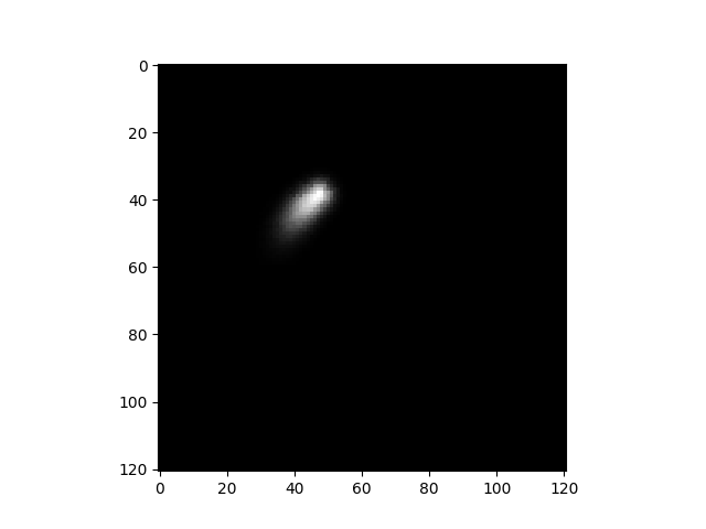
One additional feature is the _predict_spatial_jax function, which is a stripped, purely functional version of predict_percept that operates on numpy arrays. This avoids the overhead of creating p2p stimulus and percept objects, and if used correctly, provides an additional speedup.

_predict_spatial_jax takes in a (n_elecs, 3) numpy array specifying the frequency, amplitude, and pulse duration on each electrode, and two (n_elec) shaped arrays specifying the x and y locations of each electrode

model = BiphasicAxonMapModel(engine='jax')
model.build()
implant = ArgusII()
ex = np.array([implant[e].x for e in implant.electrodes])
ey = np.array([implant[e].y for e in implant.electrodes])
stim = np.zeros((60, 3))
stim[3] = [20, 1, 0.45]
percept = model._predict_spatial_jax(stim, ex, ey)
percept = np.array(percept).reshape(model.grid.shape)
plt.imshow(percept, cmap='gray')
plt.show()

One other useful feature is the predict_percept_batched function. This applies predict_percept to batches of input stimuli, using optimized matrix operations. See also its faster, stripped version _predict_spatial_batched. This function is only intended to be used if you are repeatedly simulating batches of percepts. Since jax compiles each function the first time it is used, using this function only once for a singular group of stimuli will be noticably slower than repeatedly applying predict_percept. However, splitting a very large set of stimuli into smaller batches and using predict_percept_batched will be significantly faster than predict_percept on each individual stimuli.

Note that this function consumes a large amount of memory, and may not run on systems or GPUs with limited memory.