van der Grinten, de Ruyter van Steveninck, Lozano et al. (2023): Phosphene simulation using cortical prostheses

This example shows how to apply the DynaphosModel (original and official implementation available here) to an Orion implant.

The Dynaphos model assumes that all stimuli are applied as biphasic pulse trains. Unlike other models in p2p, this model is not separated into spatial and temporal components, and must be run as a single composite model.

The model can be instantiated and run in three steps.

Creating the model

The first step is to instantiate the DynaphosModel class by calling its constructor method.

import numpy as np
import matplotlib as mpl
import matplotlib.pyplot as plt
from pulse2percept.stimuli import BiphasicPulseTrain
from pulse2percept.implants.cortex import Orion
from pulse2percept.models.cortex import DynaphosModel
model = DynaphosModel()

Parameters you don’t specify will take on default values. You can inspect all current model parameters as follows:

print(model)

DynaphosModel(a50=1.057631326853325e-07,
              a_thr=9.141886000943878e-08, dt=20,
              excitability=675, freq=300,
              grid_type='rectangular',
              kappa_trace=13.95528162, n_gray=None,
              noise=None, p_dur=0.17, regions=['v1'],
              rheobase=23.9, sig_slope=19152642.500946816,
              tau_act=111.111111, tau_trace=1967655.20573,
              verbose=True, vfmap=Polimeni2006Map,
              xrange=(-5, 5), xystep=0.25, yrange=(-5, 5))

This reveals a number of other parameters to set, such as:

• xrange, yrange: The extent of the visual field to be simulated, specified as a range of x and y coordinates (in degrees of visual angle, or dva). For example, we are currently sampling x values between -20 dva and +20dva, and y values between -15 dva and +15 dva.
• xystep: The resolution (in dva) at which to sample the visual field. For example, we are currently sampling at 0.25 dva in both x and y direction.
• dt: The time-step of the model in ms. This determines the frame-rate of the outputted percept.
• regions: The regions of the visual cortex to simulate. Currently, the Dynaphos model is only defined for the v1 region.
• freq, p_dur: The default frequency and pulse duration for the stimulus. This is used to encode a non-pulse train stimulus as a biphasic pulse train.
• excitability: The excitability constant which determines current spread, in uA/mm^2.
• rheobase: The rheobase current constant, in uA.
• tau_trace: The trace decay constant, in ms.
• kappa_trace: The stimulus effect modifier
• tau_act: The activation decay constant, in ms.
• a_thr: The tissue activation threshold, under which a phosphene is not generated. Note that this is a threshold for the internal activation value, unlike other models’ thresh_percept which is a threshold for the final percept brightness.
• sig_slope, a50: The slope of the sigmoidal brightness curve and activation value for which the brightness reaches half of its maximum.

To change parameter values, either pass them directly to the constructor above or set them by hand, like this:

model.xystep = 0.05

Then build the model. This is a necessary step before you can actually use the model to predict a percept, as it performs a number of expensive setup computations (e.g., building the grid):

model.build()

DynaphosModel(a50=1.057631326853325e-07,
              a_thr=9.141886000943878e-08, dt=20,
              excitability=675, freq=300,
              grid_type='rectangular',
              kappa_trace=13.95528162, n_gray=None,
              noise=None, p_dur=0.17, regions=['v1'],
              rheobase=23.9, sig_slope=19152642.500946816,
              tau_act=111.111111, tau_trace=1967655.20573,
              verbose=True, vfmap=Polimeni2006Map,
              xrange=(-5, 5), xystep=0.05, yrange=(-5, 5))

Important

You need to build a model only once. After that, you can apply any number of stimuli – or even apply the model to different implants – without having to rebuild (which takes time).

However, if you change important model parameters outside the constructor (e.g., by directly setting model.xystep = 0.25), you will have to call model.build() again for your changes to take effect.

Assigning a stimulus

The second step is to specify a visual prosthesis from the implants module.

In the following, we will create an Orion implant at the default location.

implant = Orion()

You can inspect the location of the implant with respect to the visual cortex using the built-in plot methods:

model.plot()
implant.plot()

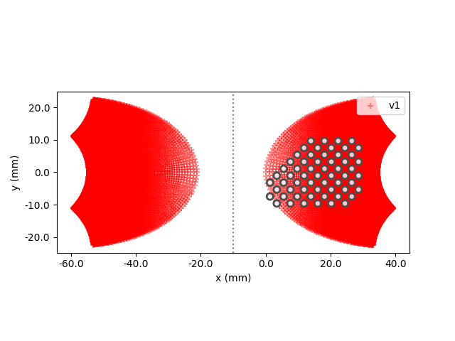
<Axes: xlabel='x (mm)', ylabel='y (mm)'>

By default, the plots will be added to the current Axes object. Alternatively, you can pass ax= to specify in which Axes to plot.

The easiest way to assign a stimulus to the implant is to pass a NumPy array that specifies the current amplitude to be applied to every electrode in the implant.

Note that all stimuli passed to Dynaphos must have a time component.

For example, the following sends 100 microamps to all electrodes of the implant, at 300Hz with a phase duration of 0.17ms:

stim_freq = 300  # stimulus frequency (Hz)
phase_dur = 0.17  # duration of the cathodic/anodic phase (ms)
stim_dur = 2000  # stimulus duration (ms)
stim_amp = 100  # stimulus current (uA)
implant.stim = {e: BiphasicPulseTrain(amp=stim_amp, freq=stim_freq,
                                      phase_dur=phase_dur, stim_dur=stim_dur)
                for e in implant.electrode_names}

Predicting the percept

The third step is to apply the model to predict the percept resulting from the specified stimulus. Note that this may take some time on your machine:

percept = model.predict_percept(implant)

The output of the model is a Percept object that contains a time series with the predicted brightness of the visual percept at every time step.

We can view the brightest frame as follows:

brightest_frame = percept.max(axis='frames')
plt.imshow(brightest_frame, cmap='gray')

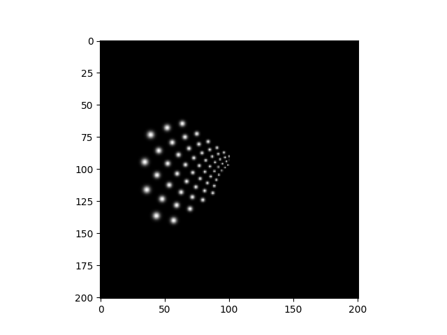
<matplotlib.image.AxesImage object at 0x7f04fd41cd90>

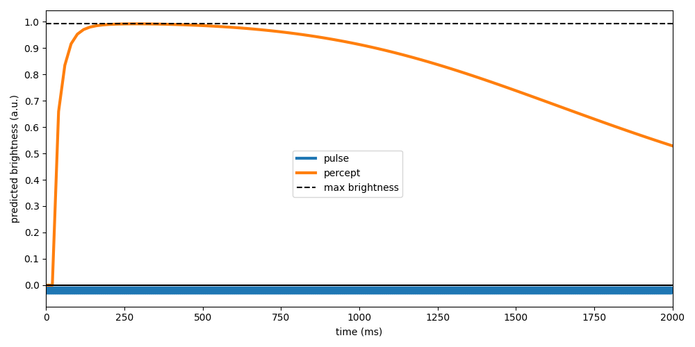
Plotting the percept-over-time next to the applied stimulus reveals that the model predicts the perceived brightness to increase rapidly and then drop off slowly (over the time course of seconds).

fig, ax = plt.subplots(figsize=(10, 5))
ax.plot(implant.stim.time,
        -0.02 + 0.01 * implant.stim.data[0, :] / implant.stim.data.max(),
        linewidth=3, label='pulse')
ax.plot(percept.time, np.max(np.max(percept.data, axis=1), axis=0), linewidth=3, label='percept')
ax.plot([0, stim_dur], [percept.max(), percept.max()], 'k--', label='max brightness')
ax.plot([0, stim_dur], [0, 0], 'k')

ax.set_xlabel('time (ms)')
ax.set_ylabel('predicted brightness (a.u.)')
ax.set_yticks(np.arange(0, 1.01, 0.1))
ax.set_xlim(0, stim_dur)
fig.legend(loc='center')
fig.tight_layout()

Brightness as a function of amplitude

The paper reports that phosphene brightness is affected by amplitude modulation.

# Use the amplitude values from the paper:
amps = [10, 20, 30, 40, 50, 60, 70, 80, 90, 100]

# Output brightness in 20ms time steps for 700ms:
t_percept = np.arange(0, 700, 20)

# Initialize an empty list that will contain the brightness-over-time
# For each amplitude
bright_over_time = []

for amp in amps:
    # For each value in the `amps` vector, now stored as `amp`, do:
    # 1. Generate a pulse train with amplitude `amp`, frequency 300Hz,
    #    166ms duration, and pulse duration 0.17ms
    implant.stim = { e: BiphasicPulseTrain(freq=300, amp=amp, phase_dur=0.17,
                                      stim_dur=166)
                    for e in implant.electrode_names }
    # 2. Run the model:
    percept = model.predict_percept(implant, t_percept=t_percept)
    # 3. Save the brightness over time
    bright_over_time.append(np.max(np.max(percept.data, axis=1), axis=0))

This allows us to reproduce the brightness-over-time plot in Fig. 3:

fig, ax = plt.subplots(1, figsize=(7.5,3))

cmap = mpl.cm.YlOrBr
norm = mpl.colors.Normalize(vmin=0, vmax=100)
fig.colorbar(None,ax=ax,cmap=cmap,norm=norm,shrink=0.5,orientation='vertical',ticks=[0,100],label="Stim. Amplitude (uA)")

ax.set_yticks([0.2, 0.6, 1.0])
ax.set_xticks([0.0, 0.2, 0.4, 0.6])
ax.set_ylim([0,1.1])
ax.set_xlim([0,0.7])
ax.spines['top'].set_visible(False)
ax.spines['right'].set_visible(False)
ax.set(ylabel='Brightness', xlabel='Time [s]')

for i, amp in enumerate(amps):
    ax.plot(t_percept / 1000, bright_over_time[i], color=cmap(amp/100), linewidth=5)

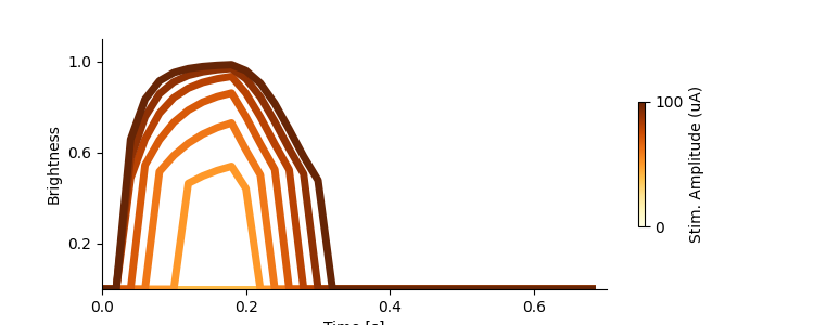
Note: For the above plot, note that we plot the generated percept brightness (which is limited by phosphene size & the tissue activation threshold) while [Grinten2023] plots the internal brightness state. The dashed lines in [Grinten2023] represent time points at which a percept is not generated, as the activation threshold was not reached.