Nanduri et al. (2012): Frequency vs. amplitude modulation

This example shows how to use the Nanduri2012Model.

The model introduced in [Nanduri2012] assumes that electrical stimulation leads to percepts that quickly increase in brightness (over the time course of ~100ms) and then slowly fade away (over the time course of seconds). The model also assumes that amplitude and frequency modulation have different effects on the perceived brightness and size of a phosphene.

Generating a pulse train

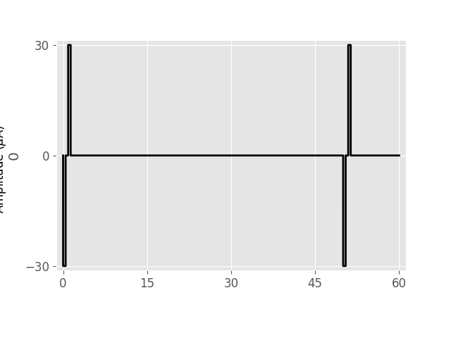
The first step is to build a pulse train using the PulseTrain class. We want to generate a 20Hz pulse train (0.45ms pulse duration, cathodic-first) at 30uA that lasts for a second:

from pulse2percept.stimuli import BiphasicPulseTrain, Stimulus
tsample = 0.005  # sampling time step (ms)
phase_dur = 0.45  # duration of the cathodic/anodic phase (ms)
stim_dur = 1000  # stimulus duration (ms)
amp_th = 30  # threshold current (uA)
stim = BiphasicPulseTrain(20, amp_th, phase_dur, interphase_dur=phase_dur,
                          stim_dur=stim_dur)

# Configure Matplotlib:
import matplotlib.pyplot as plt
plt.style.use('ggplot')
from matplotlib import rc
rc('font', size=12)

# Plot the stimulus in the range t=[0, 60] ms:
stim.plot(time=(0, 60))

<Axes: ylabel='0'>

Creating an implant

Before we can run the Nanduri model, we need to create a retinal implant to which we can assign the above pulse train.

For the purpose of this exercise, we will create an ElectrodeArray consisting of a single DiskElectrode with radius=260um centered at (x,y) = (0,0); i.e., centered over the fovea:

from pulse2percept.implants import DiskElectrode, ElectrodeArray
earray = ElectrodeArray(DiskElectrode(0, 0, 0, 260))

Usually we would use a predefined retinal implant such as ArgusII or AlphaIMS. Alternatively, we can wrap the electrode array created above with a ProsthesisSystem to create our own retinal implant. We will also assign the above created stimulus to it:

from pulse2percept.implants import ProsthesisSystem
implant = ProsthesisSystem(earray, stim=stim)

Running the model

Interacting with a model always involves three steps:

1. Initalize the model by passing the desired parameters.
2. Build the model to perform (sometimes expensive) one-time setup computations.
3. Predict the percept for a given stimulus.

In the following, we will run the Nanduri model on a single pixel, (0, 0):

from pulse2percept.models import Nanduri2012Model
model = Nanduri2012Model(xrange=(0, 0), yrange=(0, 0))
model.build()

Nanduri2012Model(asymptote=14.0, atten_a=14000,
                 atten_n=1.69, dt=0.005, engine=None,
                 eps=8.73, grid_type='rectangular',
                 n_gray=None, n_jobs=1, n_threads=2,
                 ndim=[2], noise=None, scale_out=1.0,
                 scheduler='threading', shift=16.0,
                 slope=3.0, spatial=Nanduri2012Spatial,
                 tau1=0.42, tau2=45.25, tau3=26.25,
                 temporal=Nanduri2012Temporal,
                 thresh_percept=0, verbose=True,
                 vfmap=Curcio1990Map(ndim=2),
                 xrange=(0, 0), xystep=0.25, yrange=(0, 0))

Note

You can also directly instantiate Nanduri2012Temporal and pass a stimulus to it. However, please note that there might be subtle differences; e.g., Nanduri2012Model will pass the stimulus through the spatial model first.

After building the model, we are ready to predict the percept.

The input to the model is an implant containing a stimulus (usually a pulse train), which is processed in time by a number of linear filtering steps as well as a stationary nonlinearity (a sigmoid).

import numpy as np
percept = model.predict_percept(implant, t_percept=np.arange(1000))

The output of the model is a Percept object that contains a time series with the predicted brightness of the visual percept at every time step.

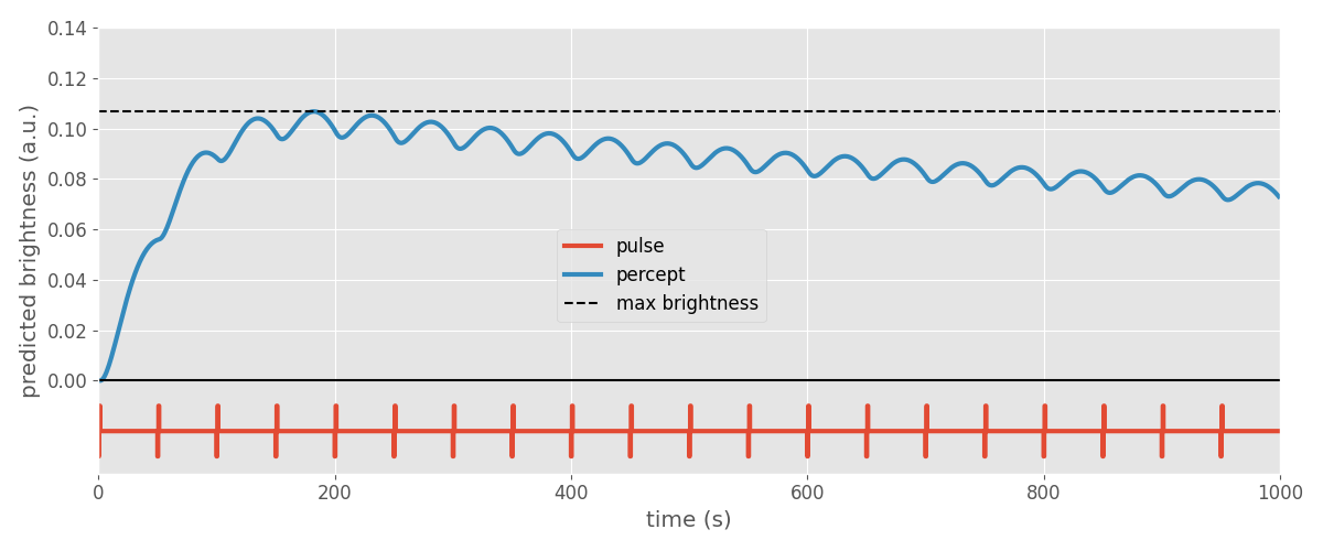
“Brightness of a stimulus” is defined as the maximum brightness value encountered over time:

bright_th = percept.data.max()
bright_th

0.10671083

Plotting the percept next to the applied stimulus reveals that the model predicts the perceived brightness to increase rapidly (within ~100ms) and then drop off slowly (over the time course of seconds). This is consistent with behavioral reports from Argus II users.

fig, ax = plt.subplots(figsize=(12, 5))
ax.plot(implant.stim.time,
        -0.02 + 0.01 * implant.stim.data[0, :] / implant.stim.data.max(),
        linewidth=3, label='pulse')
ax.plot(percept.time, percept.data[0, 0, :], linewidth=3, label='percept')
ax.plot([0, stim_dur], [bright_th, bright_th], 'k--', label='max brightness')
ax.plot([0, stim_dur], [0, 0], 'k')

ax.set_xlabel('time (s)')
ax.set_ylabel('predicted brightness (a.u.)')
ax.set_yticks(np.arange(0, 0.14, 0.02))
ax.set_xlim(0, stim_dur)
fig.legend(loc='center')
fig.tight_layout()

Note

In psychophysical experiments, brightness is usually expressed in relative terms; i.e., compared to a reference stimulus. In the model, brightness has arbitrary units.

Brightness as a function of frequency/amplitude

The Nanduri paper reports that amplitude and frequency have different effects on the perceived brightness of a phosphene.

To study these effects, we will apply the model to a number of amplitudes and frequencies:

# Use the following pulse duration (ms):
pdur = 0.45
# Generate values in the range [0, 50] uA with a step size of 5 uA or smaller:
amps = np.linspace(0, 50, 11)
# Initialize an empty list that will contain the predicted brightness values:
bright_amp = []
for amp in amps:
    # For each value in the `amps` vector, now stored as `amp`, do the
    # following:
    # 1. Generate a pulse train with amplitude `amp`, 20 Hz frequency, 0.5 s
    #    duration, pulse duration `pdur`, and interphase gap `pdur`:
    implant.stim = BiphasicPulseTrain(20, amp, pdur, interphase_dur=pdur,
                                      stim_dur=stim_dur)
    # 2. Run the temporal model:
    percept = model.predict_percept(implant)
    # 3. Find the largest value in percept, this will be the predicted
    # brightness:
    bright_pred = percept.data.max()
    # 4. Append this value to `bright_amp`:
    bright_amp.append(bright_pred)

We then repeat the procedure for a whole range of frequencies:

# Generate values in the range [0, 100] Hz with a step size of 10 Hz or
# smaller:
freqs = np.linspace(0, 100, 11)
# Initialize an empty list that will contain the predicted brightness values:
bright_freq = []
for freq in freqs:
    # For each value in the `amps` vector, now stored as `amp`, do the
    # following:
    # 1. Generate a pulse train with amplitude `amp`, 20 Hz frequency, 0.5 s
    #    duration, pulse duration `pdur`, and interphase gap `pdur`:
    implant.stim = BiphasicPulseTrain(freq, 20, pdur, interphase_dur=pdur,
                                      stim_dur=stim_dur)
    # 2. Run the temporal model
    percept = model.predict_percept(implant)
    # 3. Find the largest value in percept, this will be the predicted
    # brightness:
    bright_pred = percept.data.max()
    # 4. Append this value to `bright_amp`:
    bright_freq.append(bright_pred)

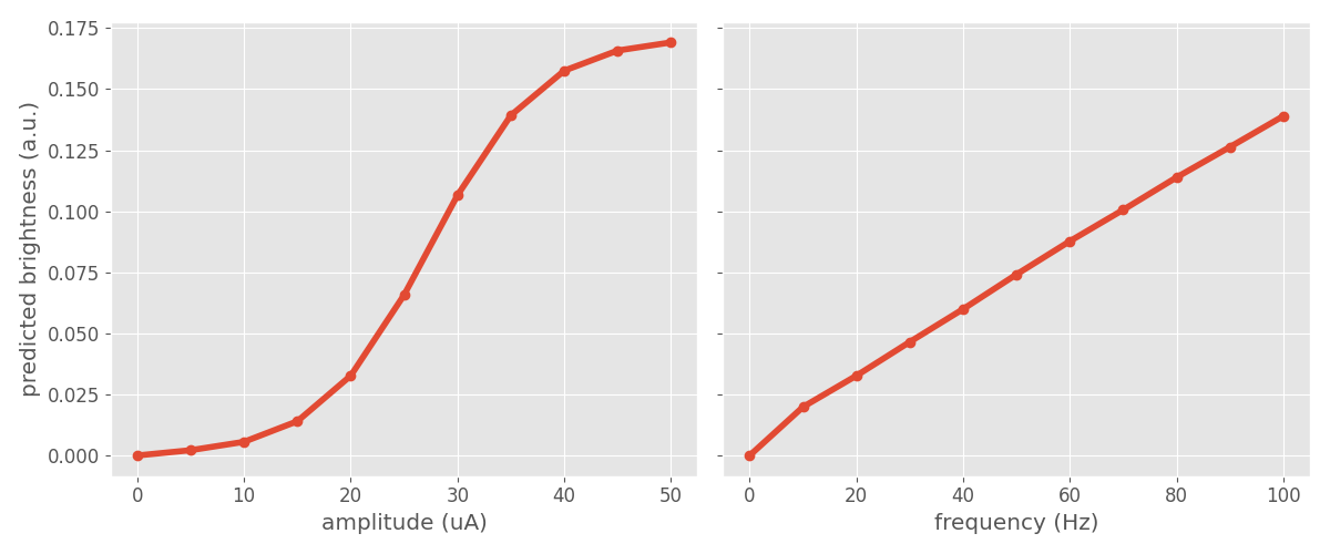
Plotting the two curves side-by-side reveals that the model predicts brightness to saturate quickly with increasing amplitude, but to scale linearly with stimulus frequency:

fig, ax = plt.subplots(ncols=2, sharey=True, figsize=(12, 5))

ax[0].plot(amps, bright_amp, 'o-', linewidth=4)
ax[0].set_xlabel('amplitude (uA)')
ax[0].set_ylabel('predicted brightness (a.u.)')

ax[1].plot(freqs, bright_freq, 'o-', linewidth=4)
ax[1].set_xlabel('frequency (Hz)')

fig.tight_layout()

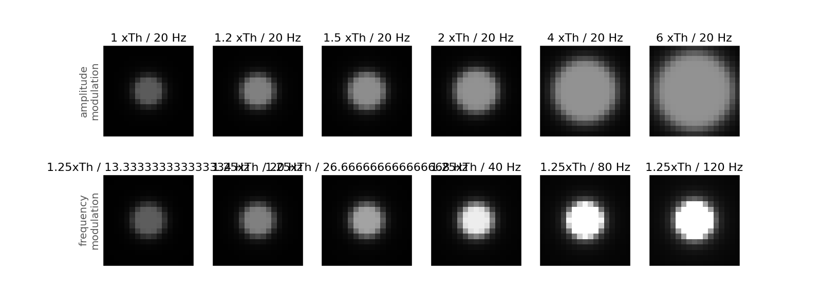
Phosphene size as a function of amplitude/frequency

The paper also reports that phosphene size is affected differently by amplitude vs. frequency modulation.

To introduce space into the model, we need to re-instantiate the model and this time provide a range of (x,y) values to simulate. These values are specified in degrees of visual angle (dva). They are sampled at xydva dva:

model = Nanduri2012Model(xystep=0.5, xrange=(-4, 4), yrange=(-4, 4))
model.build()

Nanduri2012Model(asymptote=14.0, atten_a=14000,
                 atten_n=1.69, dt=0.005, engine=None,
                 eps=8.73, grid_type='rectangular',
                 n_gray=None, n_jobs=1, n_threads=2,
                 ndim=[2], noise=None, scale_out=1.0,
                 scheduler='threading', shift=16.0,
                 slope=3.0, spatial=Nanduri2012Spatial,
                 tau1=0.42, tau2=45.25, tau3=26.25,
                 temporal=Nanduri2012Temporal,
                 thresh_percept=0, verbose=True,
                 vfmap=Curcio1990Map(ndim=2),
                 xrange=(-4, 4), xystep=0.5,
                 yrange=(-4, 4))

We will again apply the model to a whole range of amplitude and frequency values taken directly from the paper:

# Use the amplitude values from the paper:
amp_factors = [1, 1.25, 1.5, 2, 4, 6]

# Output brightness in 1ms time steps:
t_percept = np.arange(0, stim_dur, 1)

# Initialize an empty list that will contain the brightest frames:
frames_amp = []

for amp_f in amp_factors:
    # For each value in the `amp_factors` vector, now stored as `amp_f`, do:
    # 1. Generate a pulse train with amplitude `amp_f` * `amp_th`, frequency
    #    20Hz, 0.5s duration, pulse duration `pdur`, and interphase gap `pdur`:
    implant.stim = BiphasicPulseTrain(20, amp_f * amp_th, pdur,
                                      interphase_dur=pdur, stim_dur=stim_dur)
    # 2. Run the temporal model:
    percept = model.predict_percept(implant, t_percept=t_percept)
    # 3. Save the brightest frame:
    frames_amp.append(percept.max(axis='frames'))

# Use the amplitude values from the paper:
freqs = [40.0 / 3, 20, 2.0 * 40 / 3, 40, 80, 120]

# Initialize an empty list that will contain the brightest frames:
frames_freq = []

for freq in freqs:
    # For each value in the `freqs` vector, now stored as `freq`, do:
    # 1. Generate a pulse train with amplitude 1.25 * `amp_th`, frequency
    #    `freq`, 0.5s duration, pulse duration `pdur`, and interphase gap
    #    `pdur`:
    implant.stim = BiphasicPulseTrain(freq, 1.25 * amp_th, pdur,
                                      interphase_dur=pdur, stim_dur=stim_dur)
    # 2. Run the temporal model:
    percept = model.predict_percept(implant, t_percept=t_percept)
    # 3. Save the brightest frame:
    frames_freq.append(percept.max(axis='frames'))

This allows us to reproduce Fig. 7 of [Nanduri2012]:

fig, axes = plt.subplots(nrows=2, ncols=len(amp_factors), figsize=(16, 6))

for ax, amp, frame in zip(axes[0], amp_factors, frames_amp):
    ax.imshow(frame, vmin=0, vmax=0.3, cmap='gray')
    ax.set_title(f'{amp:.2g} xTh / 20 Hz', fontsize=16)
    ax.set_xticks([])
    ax.set_yticks([])
axes[0][0].set_ylabel('amplitude\nmodulation')

for ax, freq, frame in zip(axes[1], freqs, frames_freq):
    ax.imshow(frame, vmin=0, vmax=0.3, cmap='gray')
    ax.set_title(f'1.25xTh / {freq} Hz', fontsize=16)
    ax.set_xticks([])
    ax.set_yticks([])
axes[1][0].set_ylabel('frequency\nmodulation')

Text(194.44444444444446, 0.5, 'frequency\nmodulation')

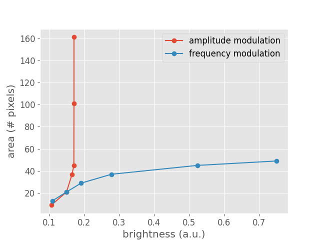
Phosphene size as a function of brightness

Lastly, the above data can also be visualized as a function of brightness to highlight the difference between frequency and amplitude modulation (see Fig.8 of [Nanduri2012]):

plt.plot([np.max(frame) for frame in frames_amp],
         [np.sum(frame >= bright_th) for frame in frames_amp],
         'o-', label='amplitude modulation')
plt.plot([np.max(frame) for frame in frames_freq],
         [np.sum(frame >= bright_th) for frame in frames_freq],
         'o-', label='frequency modulation')
plt.xlabel('brightness (a.u.)')
plt.ylabel('area (# pixels)')
plt.legend()

<matplotlib.legend.Legend object at 0x7f0592c0e530>