Beyeler et al. (2019): Axonal streaks with the axon map model

This example shows how to apply the AxonMapModel to an ArgusII implant.

The axon map model assumes that electrical stimulation leads to percepts that are elongated along the direction of the underlying nerve fiber bundle trajectory. Because the layout of nerve fiber bundles in the human retina is highly stereotyped [Jansonius2009], percept shape is predictable based on (but also highly variable depending on) the location of the stimulating electrode.

An axon’s sensitivity to electrical stimulation is assumed to decay exponentially:

• with distance from the soma \((x_{soma}, y_{soma})\), with spatial decay constant \(\lambda\),
• with distance from the stimulated retinal location \((x_{stim}, y_{stim})\), with spatial decay constant \(\rho\):

\[\begin{split}I_{axon}(x,y; \rho, \lambda) =& \exp \Big( -\frac{(x-x_{stim})^2 + (y-y_{stim})^2}{2 \rho^2} \Big) \\ & \exp \Big( -\frac{(x-x_{soma})^2 + (y-y_{soma})^2}{2 \lambda^2} \Big).\end{split}\]

The axon map model can be instantiated and run in three steps.

Creating the model

The first step is to instantiate the AxonMapModel class by calling its constructor method. The two most important parameters to set are rho and axlambda from the equation above (here set to 150 micrometers and 500 micrometers, respectively):

import numpy as np
from pulse2percept.implants import ArgusII
from pulse2percept.models import AxonMapModel
model = AxonMapModel(rho=150, axlambda=500)

Parameters you don’t specify will take on default values. You can inspect all current model parameters as follows:

print(model)

AxonMapModel(ax_segments_range=(0, 50), axlambda=500,
             axon_pickle='axons.pickle',
             axons_range=(-180, 180), engine=None,
             eye='RE', grid_type='rectangular',
             ignore_pickle=False, loc_od=(15.5, 1.5),
             min_ax_sensitivity=0.001, n_ax_segments=500,
             n_axons=1000, n_gray=None, n_jobs=1,
             n_threads=2, ndim=[2], noise=None, rho=150,
             scheduler='threading', spatial=AxonMapSpatial,
             temporal=None, thresh_percept=0, verbose=True,
             vfmap=Watson2014Map(ndim=2), xrange=(-15, 15),
             xystep=0.25, yrange=(-15, 15))

This reveals a number of other parameters to set, such as:

• xrange, yrange: the extent of the visual field to be simulated, specified as a range of x and y coordinates (in degrees of visual angle, or dva). For example, we are currently sampling x values between -20 dva and +20dva, and y values between -15 dva and +15 dva.
• xystep: The resolution (in dva) at which to sample the visual field. For example, we are currently sampling at 0.25 dva in both x and y direction.
• loc_od_x, loc_od_y: the location of the center of the optic disc (in dva)
• thresh_percept: You can also define a brightness threshold, below which the predicted output brightness will be zero. It is currently set to 1/sqrt(e), because that will make the radius of the predicted percept equal to rho.

A number of parameters control the amount of detail used when generating the axon map:

• n_axons: the number of axons to generate
• axons_range: the range of angles (in degrees) to use at which axon trajectories emanate from the center of the optic disc
• n_ax_segments: the number of segments each generated axon should have
• n_ax_segments_range: the range of distances (in dva) to use, measured from the center of the optic disc, at which axon segments should be placed
• axons_pickle: path to a pickle file where previously generated axon maps are stored

In addition, you can choose the parallelization back end used to speed up simulations:

• engine:

  • ‘serial’: single-core processing (no parallelization)
  • ‘joblib’: parallelization using the JobLib library
  • ‘dask’: parallelization using the Dask library

• scheduler:

  • ‘threading’: a scheduler backed by a thread pool
  • ‘multiprocessing’: a scheduler backed by a process pool

To change parameter values, either pass them directly to the constructor above or set them by hand, like this:

model.engine = 'serial'

Then build the model. This is a necessary step before you can actually use the model to predict a percept, as it performs a number of expensive setup computations (e.g., building the axon map, calculating electric potentials):

model.build()

AxonMapModel(ax_segments_range=(0, 50), axlambda=500,
             axon_pickle='axons.pickle',
             axons_range=(-180, 180), engine='serial',
             eye='RE', grid_type='rectangular',
             ignore_pickle=False, loc_od=(15.5, 1.5),
             min_ax_sensitivity=0.001, n_ax_segments=500,
             n_axons=1000, n_gray=None, n_jobs=1,
             n_threads=2, ndim=[2], noise=None, rho=150,
             scheduler='threading', spatial=AxonMapSpatial,
             temporal=None, thresh_percept=0, verbose=True,
             vfmap=Watson2014Map(ndim=2), xrange=(-15, 15),
             xystep=0.25, yrange=(-15, 15))

Important

You need to build a model only once. After that, you can apply any number of stimuli – or even apply the model to different implants – without having to rebuild (which takes time).

However, if you change important model parameters outside the constructor (e.g., by directly setting model.axlambda = 100), you will have to call model.build() again for your changes to take effect.

Assigning a stimulus

The second step is to specify a visual prosthesis from the implants module.

In the following, we will create an ArgusII implant. By default, the implant will be centered over the fovea (at x=0, y=0) and aligned with the horizontal meridian (rot=0):

implant = ArgusII()

You can inspect the location of the implant with respect to the underlying nerve fiber bundles using the built-in plot methods:

model.plot()
implant.plot()

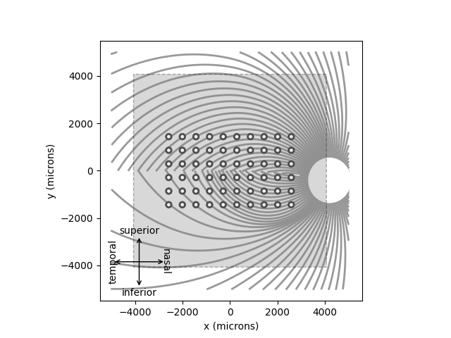
<Axes: xlabel='x (microns)', ylabel='y (microns)'>

By default, the plots will be added to the current Axes object. Alternatively, you can pass ax= to specify in which Axes to plot.

The easiest way to assign a stimulus to the implant is to pass a NumPy array that specifies the current amplitude to be applied to every electrode in the implant.

For example, the following sends 1 microamp to all 60 electrodes of the implant:

implant.stim = np.ones(60)

Predicting the percept

The third step is to apply the model to predict the percept resulting from the specified stimulus. Note that this may take some time on your machine:

percept = model.predict_percept(implant)

The resulting percept is stored in a Percept object, which is similar in organization to the Stimulus object: the data container is a 3D NumPy array (Y, X, T) with labeled axes xdva, ydva, and time.

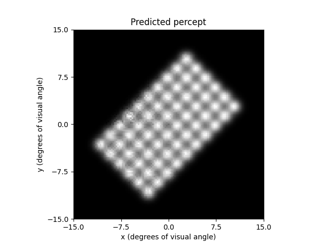
The percept can be plotted as follows:

ax = percept.plot()
ax.set_title('Predicted percept')

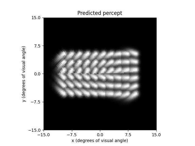
Text(0.5, 1.0, 'Predicted percept')

A major prediction of the axon map model is that the percept changes depending on the location of the implant. You can convince yourself of that by re-running the model on an implant shifted and rotated across the retina:

implant = ArgusII(x=-50, y=50, rot=-45)
model.plot()
implant.plot()

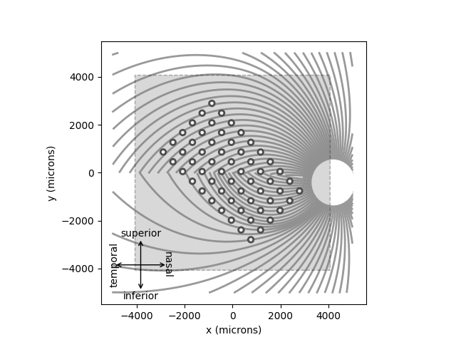
<Axes: xlabel='x (microns)', ylabel='y (microns)'>

The resulting percepts should look very different from the previous example:

implant.stim = np.ones(60)
percept = model.predict_percept(implant)
ax = percept.plot()
ax.set_title('Predicted percept')

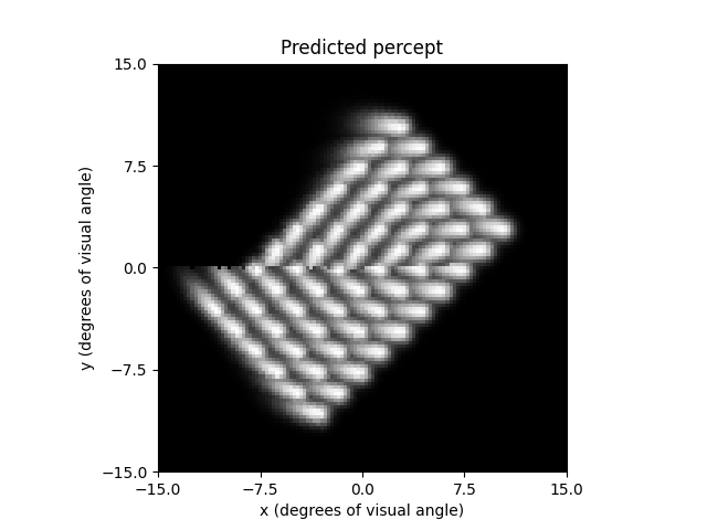
Text(0.5, 1.0, 'Predicted percept')

Important

When specifying the rotation of the implant, positive angles will result in counterclockwise rotations on the retinal surface.

However, because the superior (inferior) retina is mapped onto the lower (upper) visual field, a counterclockwise orientation on the retina is equivalent to a clockwise orientation of the percept in visual field coordinates.

You can also use the axon map model to imitate ScoreboardModel by setting lambda to a small value. However, you may have to increase the number of axons and number of segments per axon to get a smooth percept out:

model = AxonMapModel(rho=200, axlambda=10, n_axons=3000, n_ax_segments=3000)
model.build()
percept = model.predict_percept(implant)
ax = percept.plot()
ax.set_title('Predicted percept')

Text(0.5, 1.0, 'Predicted percept')

This is of course not very computationally efficient, because the model is still performing all the axon map calculations. In this case, you might be better off using ScoreboardModel.