Cortical Visual Prostheses
Visual prostheses can either be implanted on the retina or the cortex. pulse2percept was originally designed for retinal implants, but now supports cortical implants. In this section, we will cover cortical topography, implants, and models, and provide code examples of using them.
Topography
The visual cortex is the part of our brain that processes visual information. It is located at the back of our brain, and is split into two hemispheres: left and right. The visual cortex is divided into multiple regions, including v1, v2, and v3, with each region performing a different function required to process visual information.
Within a region, different parts of the visual field are processed by different neurons. We can define a mapping between locations in the visual field and locations in the cortex. This mapping is called a visual field map, also called retinotopy or visuotopy.
Model Plotting
One way to visualize the mapping between the visual field and the cortex in pulse2percept is to plot a model. A model simulates a set of points in the visual field and the corresponding points in the cortex (using a visual field map).
The first step is to create a model, for example
ScoreboardModel. We can create the
model in regions v1, v2, and v3 as follows:
In [1]: from pulse2percept.models.cortex import ScoreboardModel

In [2]: import matplotlib.pyplot as plt

In [3]: model = ScoreboardModel(regions=["v1", "v2", "v3"]).build()
Note the model.build() call. This must be called before we can plot the model.
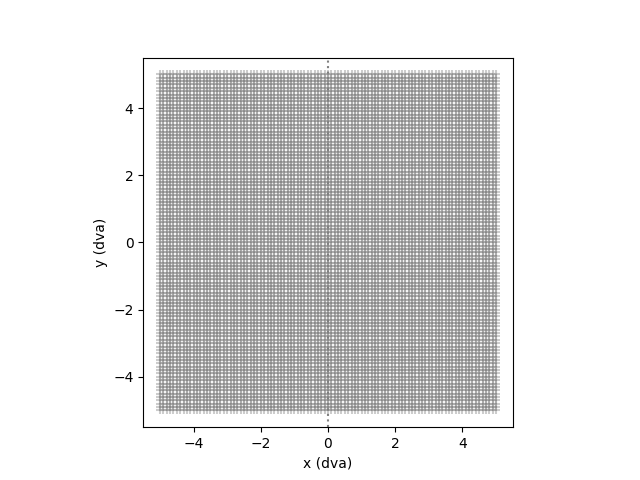
If we want to plot the model in the visual field, we can do so by setting use_dva=True. If we use the style “scatter”, then we will be able to see the points in the visual field. The points in the visual field are evenly spaced, and are represented by + symbols.
In [4]: model.plot(style="scatter", use_dva=True)
Out[4]: <Axes: xlabel='x (dva)', ylabel='y (dva)'>
If we don’t set use_dva=True, then the visual field mapping will be applied
to the points in the visual field, and the points on the cortex will be
plotted instead. ScoreboardModel by default uses the
Polimeni2006Map visual field map, but
it can also use NeuropythyMap for
3D patient-specific MRI based retinotopy.
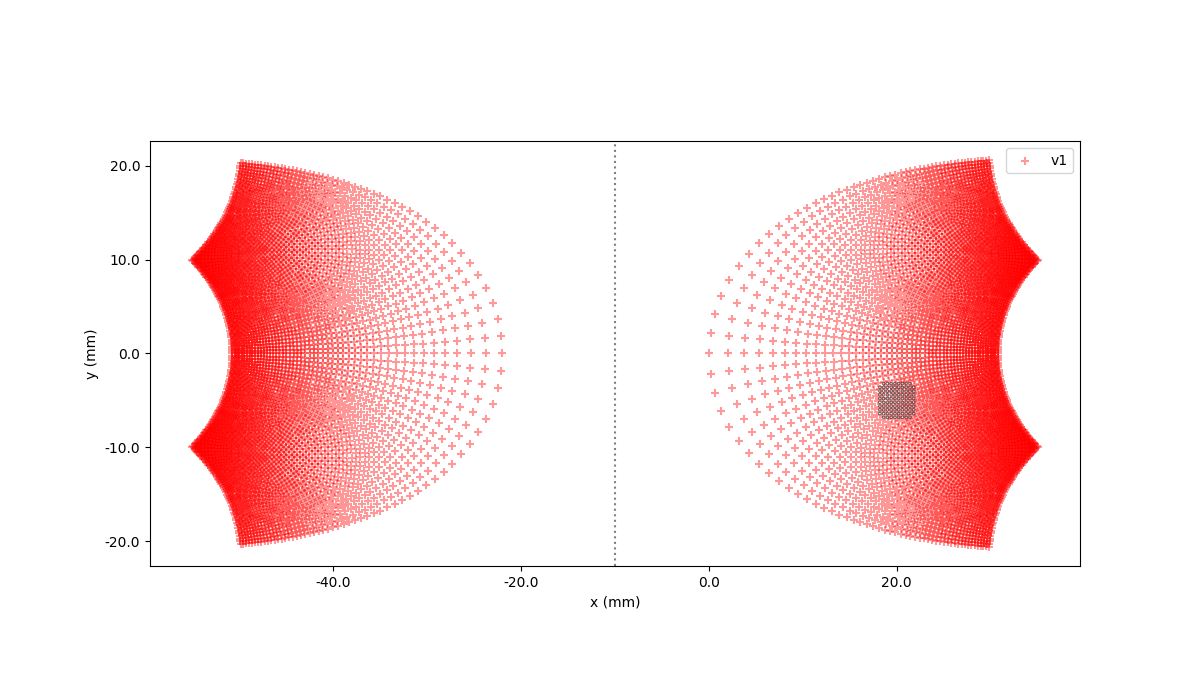
The cortex is split into left and right hemispheres, with each side being responsible for processing information from one eye. In reality, the left and right hemispheres of our brain are disconnected, but to simplify the Polimeni map represents them as one continuous space. The left hemisphere is offset by 20mm, meaning the origin of the left hemisphere is (-20000, 0). In addition, cortical visual field maps have a split_map attribute set to True, which means that no current will be allowed to cross between the hemispheres.
In [5]: model.plot(style="scatter")
Out[5]: <Axes: xlabel='x (mm)', ylabel='y (mm)'>
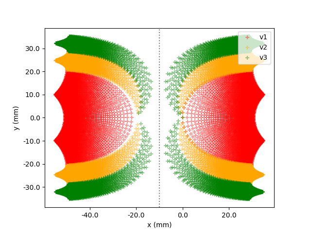
One effect that can be seen in the plot is that around the origins of each hemisphere, the points are less dense. This is because an area at the center of our visual field is represented by a larger area on the cortex than equally sized area at the periphery of our visual field, an effect called cortical magnification.
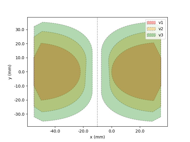
Another style option for the plot is “hull”:
In [6]: model.plot(style="hull")
Out[6]: <Axes: xlabel='x (mm)', ylabel='y (mm)'>
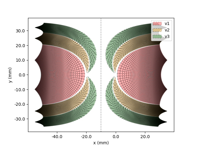
And the last style is “cell”:
In [7]: model.plot(style="cell")
Out[7]: <Axes: xlabel='x (mm)', ylabel='y (mm)'>
Visual Field Mapping Plotting
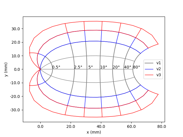
We can also directly plot visual field maps, such as
Polimeni2006Map, which is a cortical
map. The origin corresponds to the fovea (center of our visual field). The
units of the plot are in mm. The plot also shows what part of the visual
field is represented by different areas along the cortex in dva. This
shows the cortical magnification effect mentioned above, since for a given
area of the cortex near the fovea, a larger area of the visual field is
represented than the same area of the cortex near the periphery of the
visual field.
In [8]: from pulse2percept.topography import Polimeni2006Map

In [9]: map = Polimeni2006Map()

In [10]: map.plot()
Cortical Implants
Orion,
Cortivis,
and ICVP are cortical implants.
This tutorial will show you how to create and plot these implants. Setting
annotate=True will show the implant names for each electrode. The
electrode names are useful if you want to add a stimulus to specific
electrodes. For more information about these implants, see the documentation
for each specific implant.
Orion
Orion is an implant with 60
electrodes in a hex shaped grid.
In [11]: from pulse2percept.implants.cortex import Orion

In [12]: orion = Orion()

In [13]: orion.plot(annotate=True)
Out[13]: <Axes: xlabel='x (microns)', ylabel='y (microns)'>
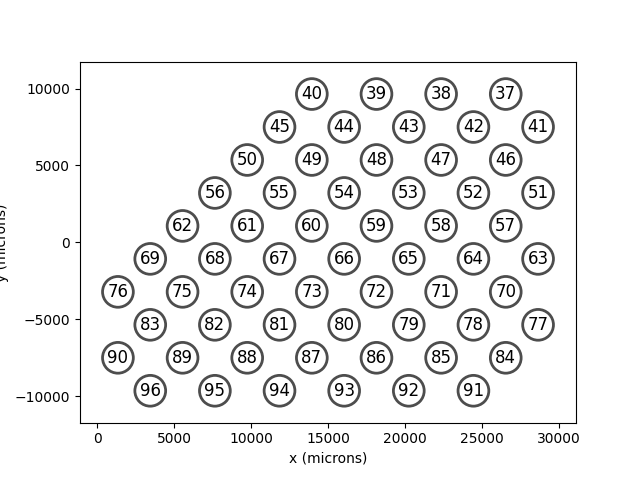
Cortivis
Cortivis is an implant with 96
electrodes in a square shaped grid.
In [14]: from pulse2percept.implants.cortex import Cortivis

In [15]: cortivis = Cortivis()

In [16]: cortivis.plot(annotate=True)
Out[16]: <Axes: xlabel='x (microns)', ylabel='y (microns)'>
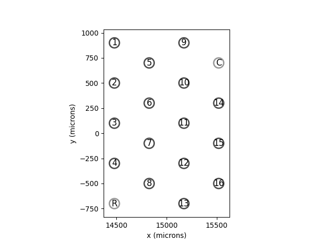
ICVP
ICVP is an implant with 16
primary electrodes in a hex shaped grid, along with 2 additional “reference”
and “counter” electrodes.
In [17]: from pulse2percept.implants.cortex import ICVP

In [18]: icvp = ICVP()

In [19]: icvp.plot(annotate=True)
Out[19]: <Axes: xlabel='x (microns)', ylabel='y (microns)'>
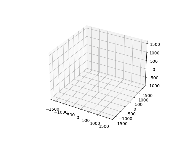
Neuralink
Neuralink is an implant
consisting of multiple Neuralink threads. Currently the only thread implemented
is the LinearEdgeThread which
consists of 32 electrodes.
In [20]: from pulse2percept.implants.cortex import LinearEdgeThread

In [21]: thread = LinearEdgeThread()

In [22]: thread.plot3D()
Out[22]: <Axes3D: >

In [23]: plt.axis('equal')
Out[23]:
(-1800.5555555555554,
 1810.5555555555554,
 -1805.5555555555554,
 1805.5555555555554,
 -1054.1666666666667,
 1654.1666666666667)
Neuralink works well with the NeuropythyMap,
which is a 3D patient-specific MRI based retinotopy. You can create
a Neuralink implant with multiple threads using the NeuropythyMap as follows:
from pulse2percept.implants.cortex import Neuralink
from pulse2percept.topography import NeuropythyMap
from pulse2percept.models.cortex import ScoreboardModel
map = NeuropythyMap('fsaverage', regions=['v1'])
model = ScoreboardModel(vfmap=map, xrange=(-4, 0), yrange=(-4, 4), xystep=.25).build()
neuralink = Neuralink.from_neuropythy(map, xrange=model.xrange, yrange=model.yrange, xystep=1, rand_insertion_angle=0)
fig = plt.figure(figsize=(10, 5))
ax1 = fig.add_subplot(121, projection='3d')
neuralink.plot3D(ax=ax1)
model.plot3D(style='cell', ax=ax1)
ax2 = fig.add_subplot(122)
neuralink.plot(ax=ax2)
model.plot(style='cell', ax=ax2)
@savefig neuralink.png align=center
plt.show()
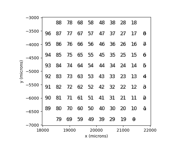
Ensemble Implants
EnsembleImplant is a new class which
allows the user to use multiple implants in tandem. It can be used with any
implant type, but was made for use with small implants meant to be used together,
such as ICVP. This tutorial will
demonstrate how to create an EnsembleImplant,
to combine multiple Cortivis objects.
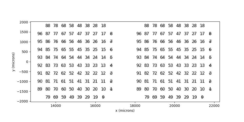
The first step is to create the individual implants that will be combined.
In [24]: i1 = Cortivis(x=15000,y=0)

In [25]: i2 = Cortivis(x=20000,y=0)

In [26]: i1.plot(annotate=True)
Out[26]: <Axes: xlabel='x (microns)', ylabel='y (microns)'>

In [27]: i2.plot(annotate=True)
Out[27]: <Axes: xlabel='x (microns)', ylabel='y (microns)'>

In [28]: plt.show()
Then, we can create an EnsembleImplant using these two implants.
In [29]: from pulse2percept.implants import EnsembleImplant

In [30]: ensemble = EnsembleImplant(implants=[i1,i2])

In [31]: _,ax = plt.subplots(1, 1, figsize=(12,7))

In [32]: ensemble.plot(annotate=True, ax=ax)
Out[32]: <Axes: xlabel='x (microns)', ylabel='y (microns)'>
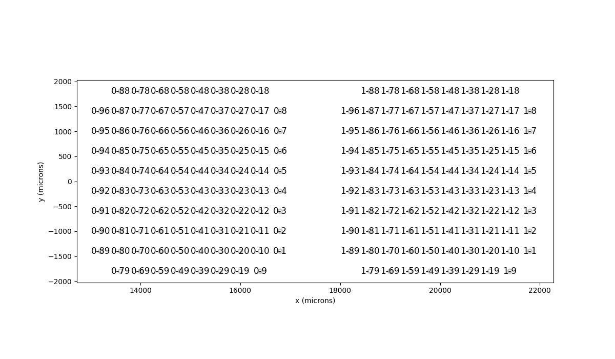
Note that electrodes are renamed, with the pattern index-electrode where index is the index of the implant in the constructor list. Implants can also be passed using a dictionary, in which case the naming pattern is key-electrode where key is the electrode’s dictionary key.
Models
This example shows how to apply the
ScoreboardModel to an
Cortivis implant.
First, we create the model and build it:
In [33]: from pulse2percept.models.cortex import ScoreboardModel

In [34]: model = ScoreboardModel(rho=1000).build()
Next, we can create the implant:
In [35]: from pulse2percept.implants.cortex import Cortivis

In [36]: implant = Cortivis()
Now, we can plot the model and implant together to see where the implant is (by default, Cortivis is centered at (15,0))
In [37]: model.plot()
Out[37]: <Axes: xlabel='x (mm)', ylabel='y (mm)'>

In [38]: implant.plot()
Out[38]: <Axes: xlabel='x (mm)', ylabel='y (mm)'>

In [39]: plt.show()
After that, we can add a stimulus to the implant. One simple way to do this is to create an array of the same shape as the implant (which has 96 electrodes), where each value in the array represents the current to apply to the corresponding electrode. For example, if we want to apply no current to the first 32 electrodes, 1 microamp of current to the next 32 electrodes, and 2 microamps of current to the last 32 electrodes, we can do the following:
In [40]: import numpy as np

In [41]: implant.stim = np.concatenate(
   ....:     (
   ....:         np.zeros(32),
   ....:         np.zeros(32) + 1,
   ....:         np.zeros(32) + 2,
   ....:     )
   ....: )
   ....:

In [42]: implant.plot(stim_cmap=True)
Out[42]: <Axes: xlabel='x (microns)', ylabel='y (microns)'>
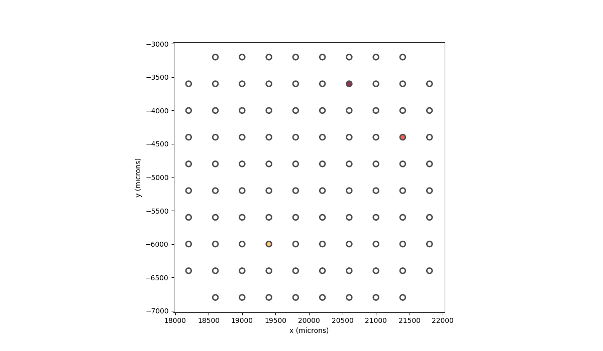
In the implant plots, darker colors indicate low current and lighter colors indicate high current (relative to the other currents). Alternatively, we can set the current for specific electrodes by passing in a dictionary, where the keys are the electrode names and the values are the current to apply to that electrode. For example, if we want to apply 1 microamp of current to the electrode named “15”, 1.5 microamps of current to the electrode named “37”, and 0.5 microamps of current to the electrode named “61”, we can do the following:
In [43]: implant.stim = {"15": 1, "37": 1.5, "61": 0.5}

In [44]: implant.plot(stim_cmap=True)
Out[44]: <Axes: xlabel='x (microns)', ylabel='y (microns)'>
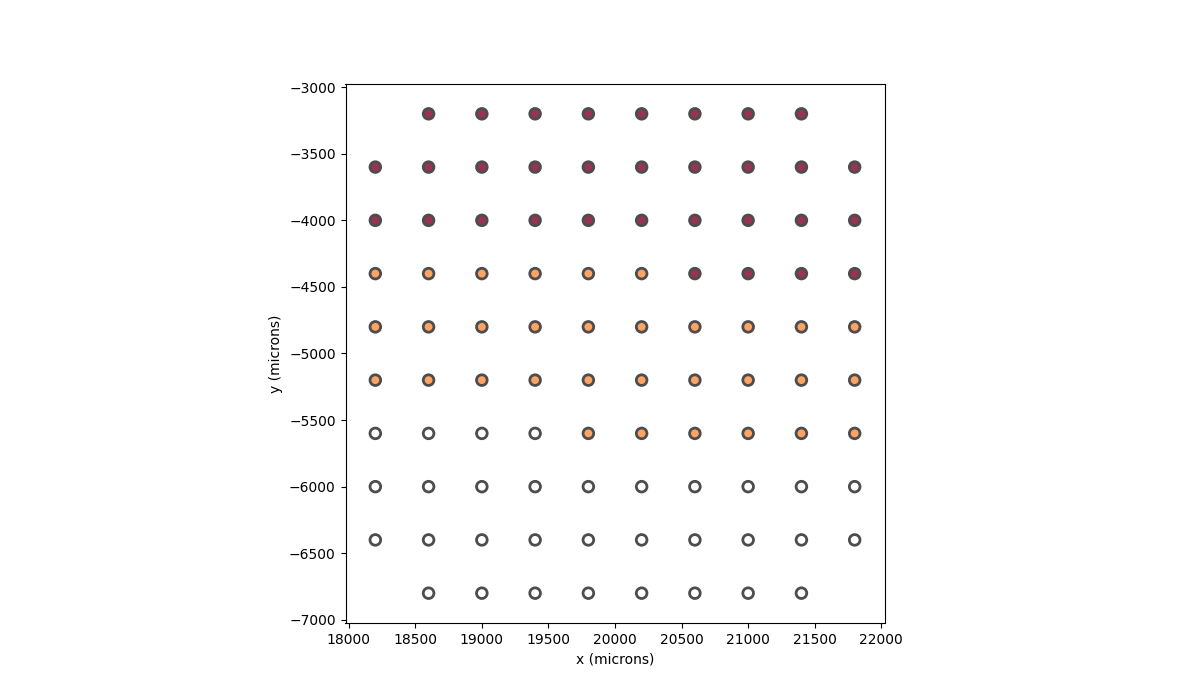
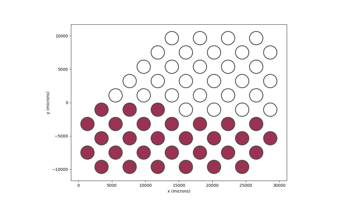
In order to make the stimulus more visible, we can use the larger
Orion implant instead.
We can add a current to the top 30 electrodes as follows:
In [45]: from pulse2percept.implants.cortex import Orion

In [46]: implant = Orion()

In [47]: implant.stim = np.concatenate(
   ....:     (
   ....:         np.zeros(30),
   ....:         np.zeros(30) + 1,
   ....:     )
   ....: )
   ....:

In [48]: implant.plot(stim_cmap=True)
Out[48]: <Axes: xlabel='x (microns)', ylabel='y (microns)'>
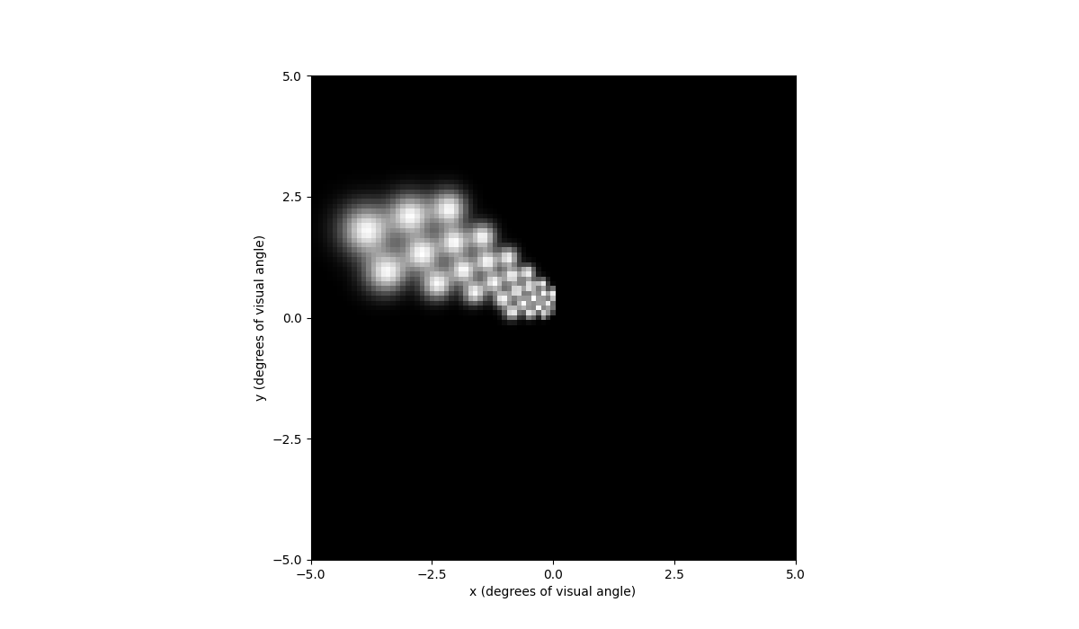
The final step is to run the model using predict_percept. This will return the calculated brightness at each location in the grid. We can then plot the brightness using the plot function:
In [49]: percept = model.predict_percept(implant)

In [50]: percept.plot()
Out[50]: <Axes: xlabel='x (degrees of visual angle)', ylabel='y (degrees of visual angle)'>
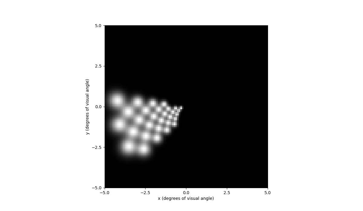
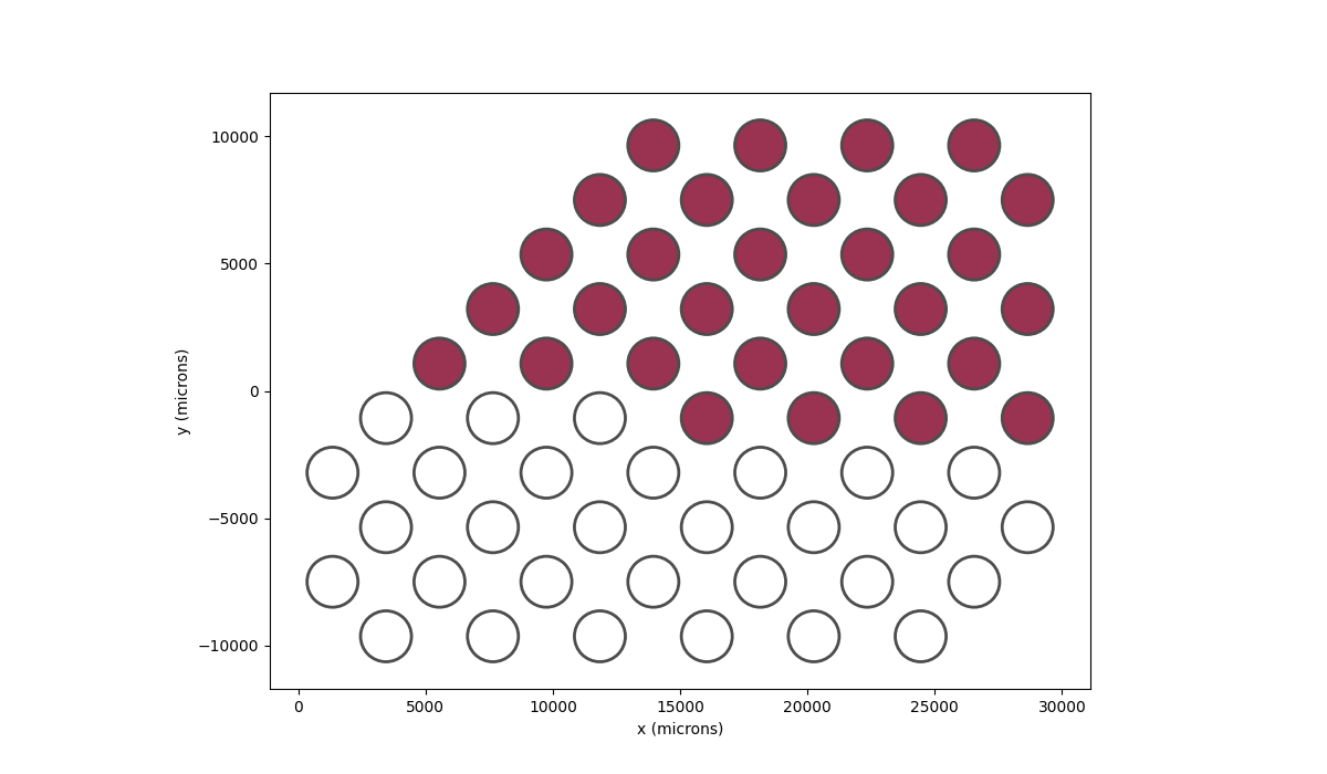
The plot shows that the top half of the visual field has brightness. If we instead stimulate the bottom 30 electrodes:
In [51]: implant.stim = np.concatenate(
   ....:     (
   ....:         np.zeros(30) + 1,
   ....:         np.zeros(30),
   ....:     )
   ....: )
   ....:

In [52]: implant.plot(stim_cmap=True)
Out[52]: <Axes: xlabel='x (microns)', ylabel='y (microns)'>
Then we will see that the bottom half of the visual field has brightness instead.
In [53]: percept = model.predict_percept(implant)

In [54]: percept.plot()
Out[54]: <Axes: xlabel='x (degrees of visual angle)', ylabel='y (degrees of visual angle)'>
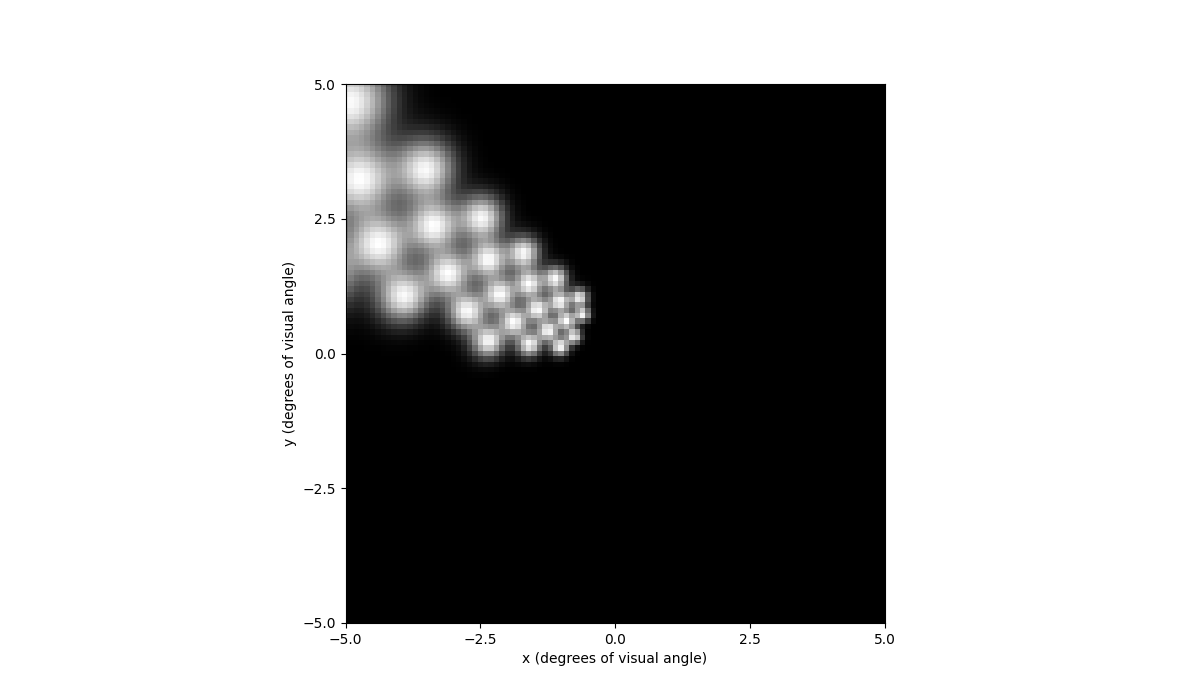
If we move the implant closer to the periphery of the visual field, we can see that the predicted percept is now larger due to cortical magnification:
In [55]: implant = Orion(x=25000)

In [56]: implant.stim = np.concatenate(
   ....:     (
   ....:         np.zeros(30) + 1,
   ....:         np.zeros(30),
   ....:     )
   ....: )
   ....:

In [57]: percept = model.predict_percept(implant)

In [58]: percept.plot()
Out[58]: <Axes: xlabel='x (degrees of visual angle)', ylabel='y (degrees of visual angle)'>
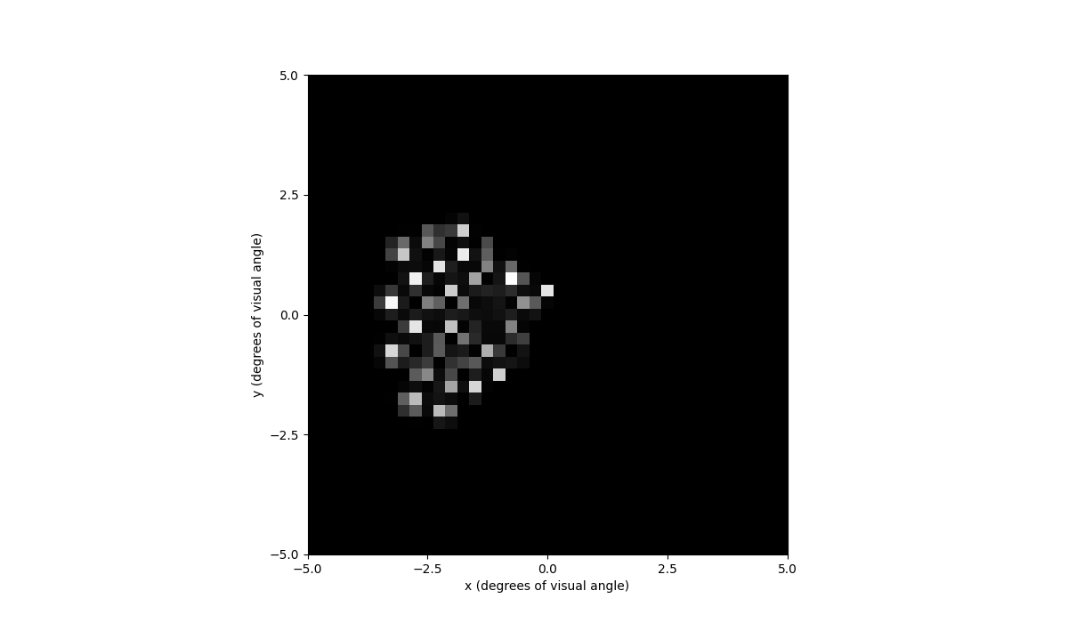
Pulse2percept currently has 2 cortical models, ScoreboardModel
and DynaphosModel. The ScoreboardModel
is a simple model that assumes that each electrode creates a circular patch of
brightness. The DynaphosModel is a more complex model that takes into account
both spatial current spread and temporal effects such as charge accumulation.
In [59]: from pulse2percept.models.cortex import DynaphosModel

In [60]: from pulse2percept.stimuli import BiphasicPulseTrain

In [61]: from pulse2percept.implants.cortex import Orion

In [62]: model = DynaphosModel().build()

In [63]: implant = Orion()

In [64]: implant.stim = {e : BiphasicPulseTrain(20, 200, .45) for e in implant.electrode_names}

In [65]: percept = model.predict_percept(implant)

In [66]: percept.plot()
Out[66]: <Axes: xlabel='x (degrees of visual angle)', ylabel='y (degrees of visual angle)'>
You can also play the percept as a video with percept.play().
For Developers
In this section we will discuss some of the changes made under the hood accomadate cortical features, as well as some important notes for developers to keep in mind.
Units
Keep in mind that pulse2percept uses units of microns for length, microamps for current, and milliseconds for time.
Topography
Mappings from the visual field to cortical coordinates are implemented
as a subclass of CorticalMap,
such as Polimeni2006Map. These
classes have a split_map attribute, which is set to True by default,
meaning that no current will be allowed to cross between the hemispheres.
These classes also have a left_offset attribute, which is set to 20mm by
default, meaning that the origin of the left hemisphere is (-20, 0) to
avoid overlapping with the right hemisphere. This is visualized above in
the model plotting section.
In order to create your own visual field map, you must create a subclass of
CorticalMap, and implement the dva_to_v1
method. In addition, if your map also maps to v2 and/or v3, you must also
implement the dva_to_v2 and/or dva_to_v3 methods. Optinally, you can also
implement v1_to_dva, v2_to_dva, and/or v3_to_dva methods.
For example, if you wanted to create a map that mapped (x, y) in dva to
(x, y) in v1, (2x, 2y) in v2, and (3x, 3y) in v3, you would do the
following (note that this is not a real map, and is only used for demonstration
purposes). See
CorticalMap for an example of a real map:
from pulse2percept.topography import CorticalMap
import numpy as np

class TestMap(CorticalMap):
    # Maps an array of points x, y in dva to an array of points x, y in v1
    def dva_to_v1(self, x, y):
        return x, y

    # Maps an array of points x, y in dva to an array of points x, y in v2
    def dva_to_v2(self, x, y):
        return 2 * x, 2 * y

    # Maps an array of points x, y in dva to an array of points x, y in v3
    def dva_to_v3(self, x, y):
        return 3 * x, 3 * y

map = TestMap(regions=["v1", "v2", "v3"])

points_dva_x = np.array([0, 1, 2])
points_dva_y = np.array([3, 4, 5])

points_v1 = map.from_dva()["v1"](points_dva_x, points_dva_y)
points_v2 = map.from_dva()["v2"](points_dva_x, points_dva_y)
points_v3 = map.from_dva()["v3"](points_dva_x, points_dva_y)

print(f"Points in v1: {points_v1}")
print(f"Points in v2: {points_v2}")
print(f"Points in v3: {points_v3}")
Points in v1: (array([0, 1, 2]), array([3, 4, 5]))
Points in v2: (array([0, 2, 4]), array([ 6, 8, 10]))
Points in v3: (array([0, 3, 6]), array([ 9, 12, 15]))