Note
Go to the end to download the full example code.
Phosphene fading data from Perez Fornos et al. (2012)
This example shows how to use the Perez Fornos et al. (2012) dataset.
[PerezFornos2012] had nine Argus II users report perceived phosphene brightness via joystick position.
Important
You will need to install Pandas
(pip install pandas) for this dataset.
Loading the dataset
The dataset can be loaded as a Pandas DataFrame:
import numpy as np
import matplotlib.pyplot as plt
from pulse2percept.datasets import load_perezfornos2012

data = load_perezfornos2012()
print(data)
     figure subject                                        time_series
0   fig3_S1      S1  [nan, nan, nan, nan, 0.0, 10.289855072463762, ...
1   fig3_S2      S2  [nan, nan, nan, nan, 0.0, 9.456201550387616, 0...
2   fig3_S3      S3  [nan, nan, nan, nan, 0.0, 6.539635936582497, 9...
3   fig3_S4      S4  [nan, nan, nan, nan, 0.0, 2.759210526315784, 9...
4   fig3_S5      S5  [nan, nan, nan, nan, 0.0, 7.373643410852728, 9...
5   fig3_S6      S6  [nan, nan, nan, nan, 0.0, 9.053658536585358, 1...
6   fig3_S7      S7  [nan, nan, nan, nan, 0.0, 6.839285714285683, 1...
7   fig3_S8      S8  [nan, nan, nan, nan, 0.0, 9.966442953020133, 9...
8   fig3_S9      S9  [nan, nan, nan, nan, 0.0, 8.148230088495582, 4...
9   fig4_S1      S1  [nan, nan, nan, nan, 0.0, 9.583152173913025, 9...
10  fig4_S2      S2  [nan, nan, nan, nan, nan, 0.0885339538819553, ...
11  fig4_S3      S3  [nan, nan, nan, nan, 0.0, 9.355113636363637, 6...
12  fig4_S4      S4  [nan, nan, nan, nan, 0.0, 4.709610849056605, 9...
13  fig4_S5      S5  [nan, nan, nan, nan, 0.0, 5.867696323345818, 9...
14  fig4_S6      S6  [nan, nan, nan, nan, 0.0, 4.897842056932968, 9...
15  fig4_S7      S7  [nan, nan, nan, nan, 0.0, 10.423076923076923, ...
16  fig4_S8      S8  [nan, nan, nan, nan, 0.0, 9.825298540468818, 8...
17  fig4_s9      S9  [nan, nan, nan, nan, 0.0, 9.917355371900818, 7...
18  fig5_S1      S1  [nan, nan, nan, nan, 0.0, 6.46536796536796, 8....
19  fig5_S2      S2  [nan, nan, nan, nan, 0.0, 9.545454545454517, 0...
20  fig5_S3      S3  [nan, nan, nan, nan, 0.0, 9.252173913043483, 4...
21  fig5_S4      S4  [nan, nan, nan, nan, 0.0, 0.0, 0.5709745762711...
22  fig5_S5      S5  [nan, nan, nan, nan, 0.0, 6.098460336915207, 1...
23  fig5_S6      S6  [nan, nan, nan, nan, 0.0, 3.694806525659934, 9...
24  fig5_S7      S7  [nan, nan, nan, nan, 0.0, 7.210290722042516, 3...
25  fig5_S8      S8  [nan, nan, nan, nan, 0.0, 10.564581725133657, ...
26  fig5_S9      S9  [nan, nan, nan, nan, 0.0, 2.812601834084476, 7...
27  fig6_S1      S1  [nan, nan, nan, nan, 0.0, 9.566193845005886, 9...
28  fig6_S2      S2  [nan, nan, nan, nan, 0.0, 0.4496233521657302, ...
29  fig6_S3      S3  [nan, nan, nan, nan, nan, 7.515737410071948, 9...
30  fig6_S4      S4  [nan, nan, nan, -0.4626257135091045, -0.565371...
31  fig6_S5      S5  [nan, nan, nan, nan, nan, 7.978896103896103, 9...
32  fig6_S6      S6  [nan, nan, nan, nan, 0.0, 4.922984609602596, 6...
33  fig6_S7      S7  [nan, nan, nan, nan, 0.0, 5.908221351250469, 0...
34  fig6_S8      S8  [nan, nan, nan, nan, 0.0, 8.429239812152321, 9...
35  fig6_S9      S9  [nan, nan, nan, nan, 0.0, 6.600741633249903, 2...
36  fig7_S1      S1  [nan, nan, nan, nan, 0.0, 1.977431770468857, 3...
37  fig7_S2      S2  [nan, nan, nan, nan, 0.0, 2.0393053016453364, ...
38  fig7_S3      S3  [nan, nan, nan, nan, 0.0, 2.830743879472698, 6...
39  fig7_S4      S4  [nan, nan, nan, nan, 0.0, 1.4526049204052085, ...
40  fig7_S5      S5  [nan, nan, nan, nan, 0.0, 1.7023601398601456, ...
41  fig7_S6      S6  [nan, nan, nan, nan, 0.0, 1.719339622641511, 4...
42  fig7_S7      S7  [nan, nan, nan, nan, 0.0, 4.362728503723769, 8...
43  fig7_S8      S8  [nan, nan, nan, nan, 0.0, 3.976098776619857, 7...
44  fig7_S9      S9  [nan, nan, nan, nan, 0.0, 2.2775319567354897, ...
Inspecting the DataFrame tells us that there are 45 measurements (the rows) each with 3 different attributes (the columns).
These attributes include specifiers such as “subject”, “figure”, and “time_series”. We can print all column names using:
data.columns
Index(['figure', 'subject', 'time_series'], dtype='object')
Note
The meaning of all column names is explained in the docstring of
the load_fornos2012() function.
For example, “subject” corresponds to each subject used in the paper:
data.subject.unique()
array(['S1', 'S2', 'S3', ..., 'S7', 'S8', 'S9'], dtype=object)
To select all the rows where the subject frequency was ‘S2’, we can index into the DataFrame as follows:
print(data[data.subject == 'S2'])
     figure subject                                        time_series
1   fig3_S2      S2  [nan, nan, nan, nan, 0.0, 9.456201550387616, 0...
10  fig4_S2      S2  [nan, nan, nan, nan, nan, 0.0885339538819553, ...
19  fig5_S2      S2  [nan, nan, nan, nan, 0.0, 9.545454545454517, 0...
28  fig6_S2      S2  [nan, nan, nan, nan, 0.0, 0.4496233521657302, ...
37  fig7_S2      S2  [nan, nan, nan, nan, 0.0, 2.0393053016453364, ...
However, we can do the same operation when loading in the data as follows:
print(load_perezfornos2012(subjects='S2'))
    figure subject                                        time_series
0  fig3_S2      S2  [nan, nan, nan, nan, 0.0, 9.456201550387616, 0...
1  fig4_S2      S2  [nan, nan, nan, nan, nan, 0.0885339538819553, ...
2  fig5_S2      S2  [nan, nan, nan, nan, 0.0, 9.545454545454517, 0...
3  fig6_S2      S2  [nan, nan, nan, nan, 0.0, 0.4496233521657302, ...
4  fig7_S2      S2  [nan, nan, nan, nan, 0.0, 2.0393053016453364, ...
This leaves us with 4 rows, each pertaining to subject ‘S2’.
Note
Please see the documentation for
load_perezfornos2012() to see all
available parameters for data subset loading.
Plotting the data
One of the important points in the paper is how the perceptual response varies amongst subjects. Let us recreate Figure 3, for Subject 2, to show an example of this difference:
# Load in each figures data:
figure_3_s1_data = load_perezfornos2012(figures='fig3_S1')['time_series'][0]
figure_3_s2_data = load_perezfornos2012(figures='fig3_S2')['time_series'][0]
Stimuli were delivered over a 10 second window. To recreate this, we build
a vector of time points (time_steps) and set stimulation value to 10
within the first 10 seconds, and 0 otherwise:
time_steps = np.arange(start=-2.0, stop=75.5, step=0.5)

# Set up the pulse:
pulse_value = []
for pulse_step in time_steps:
    if 10 >= pulse_step > 0:
        pulse_value.append(10)
    else:
        pulse_value.append(0)
Now we can plot the stimulus alongside the subject’s response:
# Set up the subplot:
fig, (ax1, ax2) = plt.subplots(1, 2, sharex=True, sharey=True)
plt.xlim(-1, 30)
plt.ylim(-11, 11)
fig.suptitle('Average Joystick Response vs. Time')

# Plot subject 1
ax1.plot(time_steps, figure_3_s1_data, 'r', label='S1 Joystick Response')
ax1.step(time_steps, pulse_value, 'k--', label='Pulse')
ax1.spines['bottom'].set_position('center')
ax1.set_title('S1')
ax1.legend(loc='lower right')

# Plot subject 2
ax2.plot(time_steps, figure_3_s2_data, label='S2 Joystick Response')
ax2.step(time_steps, pulse_value, 'k--', label='Pulse')
ax2.spines['bottom'].set_position('center')
ax2.set_title('S2')
ax2.legend(loc='lower right')

fig.tight_layout()
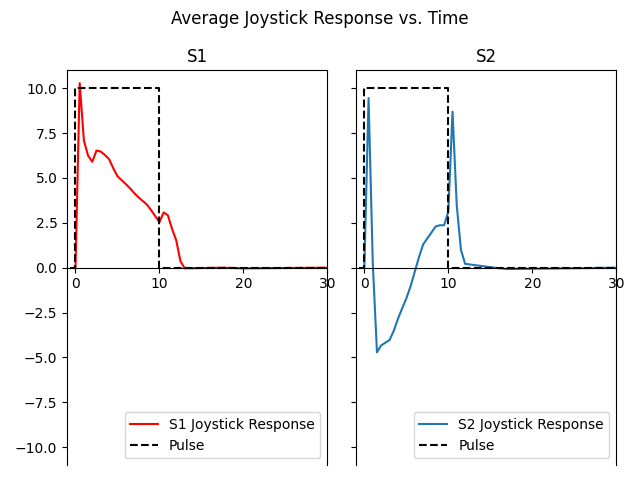
The above plot suggests that Subject 1 saw phosphenes gradually get dimmer over the stimulus duration. Once the stimulus was removed, phosphene brightness was quickly reduced to zero.
For Subject 2, the phosphene started bright (t=0) but rapidly went dark, even darker than the background (y-value < 0). Then the phosphene slowly got brighter again. Upon stimulus removal, the subject reported seeing another flash of light.
The reason for these differences is currently unknown, but might have to do with retinal adaptation.
Total running time of the script: (0 minutes 0.198 seconds)