Note
Go to the end to download the full example code.
Data from Nanduri et al. (2012)
This example shows how to use the Nanduri et al. (2012) dataset.
[Nanduri2012] used a set of psychophysical detection tasks to determine size and brightness of phosphenes by modulating current amplitude and stimulating frequency in one Argus I user.
Important
You will need to install Pandas
(pip install pandas) for this dataset.
Loading the dataset
The dataset can be loaded as a Pandas DataFrame:
from pulse2percept.datasets import load_nanduri2012
data = load_nanduri2012()
print(data)
    subject implant electrode  ... interphase_dur     pulse_type  varied_param
0       S06  ArgusI        A2  ...           0.45  cathodicfirst           amp
1       S06  ArgusI        A2  ...           0.45  cathodicfirst           amp
2       S06  ArgusI        A2  ...           0.45  cathodicfirst           amp
3       S06  ArgusI        A2  ...           0.45  cathodicfirst           amp
4       S06  ArgusI        A2  ...           0.45  cathodicfirst           amp
..      ...     ...       ...  ...            ...            ...           ...
123     S06  ArgusI        D4  ...           0.45  cathodicfirst           amp
124     S06  ArgusI        D4  ...           0.45  cathodicfirst           amp
125     S06  ArgusI        D4  ...           0.45  cathodicfirst           amp
126     S06  ArgusI        D4  ...           0.45  cathodicfirst           amp
127     S06  ArgusI        D4  ...           0.45  cathodicfirst           amp

[128 rows x 17 columns]
Inspecting the DataFrame tells us that there are 128 measurements (the rows) each with 17 different attributes (the columns).
These attributes include specifiers such as “subject”, “electrode”, and “freq”. We can print all column names using:
data.columns
Index(['subject', 'implant', 'electrode', 'task', 'stim_class', 'stim_dur',
       'freq', 'amp_factor', 'ref_stim_class', 'ref_amp_factor', 'ref_freq',
       'brightness', 'size', 'pulse_dur', 'interphase_dur', 'pulse_type',
       'varied_param'],
      dtype='object')
Note
The meaning of all column names is explained in the docstring of
the load_nanduri2012() function.
For example, “freq” corresponds to the different stimulation frequency (hz) that were used in the paper:
data.freq.unique()
array([ 20., 15., 25., 40., 80., 120.])
To select all the rows where the stimulation frequency was 20hz, we can index into the DataFrame as follows:
print(data[data.freq == 20.0])
    subject implant electrode  ... interphase_dur     pulse_type  varied_param
0       S06  ArgusI        A2  ...           0.45  cathodicfirst           amp
1       S06  ArgusI        A2  ...           0.45  cathodicfirst           amp
2       S06  ArgusI        A2  ...           0.45  cathodicfirst           amp
3       S06  ArgusI        A2  ...           0.45  cathodicfirst           amp
4       S06  ArgusI        A2  ...           0.45  cathodicfirst           amp
..      ...     ...       ...  ...            ...            ...           ...
123     S06  ArgusI        D4  ...           0.45  cathodicfirst           amp
124     S06  ArgusI        D4  ...           0.45  cathodicfirst           amp
125     S06  ArgusI        D4  ...           0.45  cathodicfirst           amp
126     S06  ArgusI        D4  ...           0.45  cathodicfirst           amp
127     S06  ArgusI        D4  ...           0.45  cathodicfirst           amp

[88 rows x 17 columns]
This leaves us with 88 rows.
One of the important points of the paper is to investigate the relationship between phosphene brightness and size as either the stimulation amplitude factor or frequency varies. We can easily load in all data points where phosphene brightness was recorded when initially loading in the data set.
print(load_nanduri2012(task='rate'))
   subject implant electrode  ... interphase_dur     pulse_type  varied_param
0      S06  ArgusI        A2  ...           0.45  cathodicfirst           amp
1      S06  ArgusI        A2  ...           0.45  cathodicfirst           amp
2      S06  ArgusI        A2  ...           0.45  cathodicfirst           amp
3      S06  ArgusI        A2  ...           0.45  cathodicfirst           amp
4      S06  ArgusI        A2  ...           0.45  cathodicfirst           amp
..     ...     ...       ...  ...            ...            ...           ...
83     S06  ArgusI        D4  ...           0.45  cathodicfirst          freq
84     S06  ArgusI        D4  ...           0.45  cathodicfirst          freq
85     S06  ArgusI        D4  ...           0.45  cathodicfirst          freq
86     S06  ArgusI        D4  ...           0.45  cathodicfirst          freq
87     S06  ArgusI        D4  ...           0.45  cathodicfirst          freq

[88 rows x 17 columns]
Likewise, we can load in all data points where phosphene size was recorded when initially loading in the data set.
print(load_nanduri2012(task='size'))
   subject implant electrode  ... interphase_dur     pulse_type  varied_param
0      S06  ArgusI        A2  ...           0.45  cathodicfirst           amp
1      S06  ArgusI        A2  ...           0.45  cathodicfirst           amp
2      S06  ArgusI        A2  ...           0.45  cathodicfirst           amp
3      S06  ArgusI        A2  ...           0.45  cathodicfirst           amp
4      S06  ArgusI        A2  ...           0.45  cathodicfirst           amp
5      S06  ArgusI        A4  ...           0.45  cathodicfirst           amp
6      S06  ArgusI        A4  ...           0.45  cathodicfirst           amp
7      S06  ArgusI        A4  ...           0.45  cathodicfirst           amp
8      S06  ArgusI        A4  ...           0.45  cathodicfirst           amp
9      S06  ArgusI        A4  ...           0.45  cathodicfirst           amp
10     S06  ArgusI        B1  ...           0.45  cathodicfirst           amp
11     S06  ArgusI        B1  ...           0.45  cathodicfirst           amp
12     S06  ArgusI        B1  ...           0.45  cathodicfirst           amp
13     S06  ArgusI        B1  ...           0.45  cathodicfirst           amp
14     S06  ArgusI        B1  ...           0.45  cathodicfirst           amp
15     S06  ArgusI        C1  ...           0.45  cathodicfirst           amp
16     S06  ArgusI        C1  ...           0.45  cathodicfirst           amp
17     S06  ArgusI        C1  ...           0.45  cathodicfirst           amp
18     S06  ArgusI        C1  ...           0.45  cathodicfirst           amp
19     S06  ArgusI        C1  ...           0.45  cathodicfirst           amp
20     S06  ArgusI        C4  ...           0.45  cathodicfirst           amp
21     S06  ArgusI        C4  ...           0.45  cathodicfirst           amp
22     S06  ArgusI        C4  ...           0.45  cathodicfirst           amp
23     S06  ArgusI        C4  ...           0.45  cathodicfirst           amp
24     S06  ArgusI        C4  ...           0.45  cathodicfirst           amp
25     S06  ArgusI        D2  ...           0.45  cathodicfirst           amp
26     S06  ArgusI        D2  ...           0.45  cathodicfirst           amp
27     S06  ArgusI        D2  ...           0.45  cathodicfirst           amp
28     S06  ArgusI        D2  ...           0.45  cathodicfirst           amp
29     S06  ArgusI        D2  ...           0.45  cathodicfirst           amp
30     S06  ArgusI        D3  ...           0.45  cathodicfirst           amp
31     S06  ArgusI        D3  ...           0.45  cathodicfirst           amp
32     S06  ArgusI        D3  ...           0.45  cathodicfirst           amp
33     S06  ArgusI        D3  ...           0.45  cathodicfirst           amp
34     S06  ArgusI        D3  ...           0.45  cathodicfirst           amp
35     S06  ArgusI        D4  ...           0.45  cathodicfirst           amp
36     S06  ArgusI        D4  ...           0.45  cathodicfirst           amp
37     S06  ArgusI        D4  ...           0.45  cathodicfirst           amp
38     S06  ArgusI        D4  ...           0.45  cathodicfirst           amp
39     S06  ArgusI        D4  ...           0.45  cathodicfirst           amp

[40 rows x 17 columns]
Note
Please see the documentation for load_nanduri2012()
to see all available parameters for data subset loading.
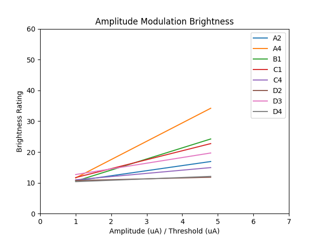
Plotting the data
To see the relationship between phosphene brightness as the amplitude factor varies,
we can recreate figure 4 a, from the paper.
Furthermore, the dataset available in load_nanduri2012()
is used to create figures 4 and 5, a-d in the paper.
import matplotlib.pyplot as plt
import numpy as np

# load subset of the dataset concerning brightness data
brightness_data = load_nanduri2012(task='rate')

# get data where stimulation amplitude is varied
vary_amp = brightness_data[brightness_data.varied_param == 'amp']

# get the list of electrodes
electrodes = data['electrode'].unique()

# iterate over all electrodes
for electrode in electrodes:
    # get relevant data for this specific electrode
    electrode_data = vary_amp[vary_amp.electrode == electrode]

    # normalize the amplitude
    normalized_amp = electrode_data.amp_factor / electrode_data.ref_amp_factor

    # set brightness rating
    brightness_rating = electrode_data.brightness

    # perform a first order linear best fit
    linear_fit = np.poly1d(np.polyfit(normalized_amp, brightness_rating, 1))

    # plot the linear best fit
    plt.plot(normalized_amp, linear_fit(normalized_amp), label=electrode)

# display legend on plot
plt.legend()

# set plot axes
plt.xlim(0, 7)
plt.ylim(0, 60)

# set plot labels and title
plt.xlabel('Amplitude (uA) / Threshold (uA)')
plt.ylabel('Brightness Rating')
plt.title('Amplitude Modulation Brightness')
Text(0.5, 1.0, 'Amplitude Modulation Brightness')
Using Built-In Plotting Functionality
Arguably the most important column is “freq”. This is the current amplitude of the different stimuli (single pulse, pulse trains, etc.) used at threshold.
We might be interested in seeing how the phosphene brightness varies as a function of pulse frequency. We could either use Matplotlib to generate a scatter plot or use pulse2percept’s own visualization function:
from pulse2percept.viz import scatter_correlation
scatter_correlation(data.freq, data.brightness)
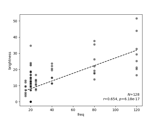
<Axes: xlabel='freq', ylabel='brightness'>
scatter_correlation() above generates a scatter
plot of the phosphene brightness as a function of pulse frequency, and performs
linear regression to calculate a correlation $r$ and a $p$ value.
As expected from the literature, now it becomes evident that phosphene
brightness is positively correlated with pulse frequency
Total running time of the script: (0 minutes 0.145 seconds)