Note
Go to the end to download the full example code.
Phosphene drawings from Beyeler et al. (2019)
This example shows how to use the Beyeler et al. (2019) dataset.
[Beyeler2019] asked Argus I/II users to draw what they see in response to single-electrode stimulation.
Important
For this dataset you will need to install both
Pandas (pip install pandas) and
HDF4 for Python (pip install h5py).
Loading the dataset
Due to its size (66 MB), the dataset is not included with pulse2percept, but can be downloaded from the Open Science Framework (OSF).
By default, the dataset will be stored in a local directory ‘~/pulse2percept_data/’ within your user directory (but a different path can be specified). This way, the datasets is only downloaded once, and future calls to the fetch function will load the dataset from your local copy.
The data itself will be provided as a Pandas DataFrame:
from pulse2percept.datasets import fetch_beyeler2019

data = fetch_beyeler2019()
print(data)
    subject  amp   area  ...  implant_rot         xrange         yrange
0        S1  2.0   1614  ...       -64.74  (-36.9, 36.9)  (-36.9, 36.9)
1        S1  2.0   3691  ...       -64.74  (-36.9, 36.9)  (-36.9, 36.9)
2        S1  2.0   1812  ...       -64.74  (-36.9, 36.9)  (-36.9, 36.9)
3        S1  2.0   1970  ...       -64.74  (-36.9, 36.9)  (-36.9, 36.9)
4        S1  2.0   1554  ...       -64.74  (-36.9, 36.9)  (-36.9, 36.9)
..      ...  ...    ...  ...          ...            ...            ...
395      S4  2.0    902  ...       -34.00      (-32, 32)      (-24, 24)
396      S4  2.0   8312  ...       -34.00      (-32, 32)      (-24, 24)
397      S4  2.0   8754  ...       -34.00      (-32, 32)      (-24, 24)
398      S4  2.0    888  ...       -34.00      (-32, 32)      (-24, 24)
399      S4  2.0  12954  ...       -34.00      (-32, 32)      (-24, 24)

[400 rows x 26 columns]
Inspecting the DataFrame tells us that there are 400 phosphene drawings (the rows) each with 16 different attributes (the columns).
These attributes include specifiers such as “subject”, “electrode”, and “image”. We can print all column names using:
data.columns
Index(['subject', 'amp', 'area', 'compactness', 'date', 'eccentricity',
       'electrode', 'filename', 'freq', 'image', 'orientation', 'pdur',
       'stim_class', 'x_center', 'xrange_x', 'xrange_y', 'y_center',
       'yrange_x', 'yrange_y', 'img_shape', 'implant_type_str', 'implant_x',
       'implant_y', 'implant_rot', 'xrange', 'yrange'],
      dtype='object')
Note
The meaning of all column names is explained in the docstring of
the fetch_beyeler2019() function.
For example, “subject” contains the different subject IDs used in the study:
data.subject.unique()
array(['S1', 'S2', 'S3', 'S4'], dtype=object)
To select all drawings from Subject 2, we can index into the DataFrame as follows:
print(data[data.subject == 'S2'])
    subject  amp  area  ...  implant_rot     xrange         yrange
60       S2  2.0   548  ...        -44.0  (-30, 30)  (-22.5, 22.5)
61       S2  2.0  7875  ...        -44.0  (-30, 30)  (-22.5, 22.5)
62       S2  2.0  4494  ...        -44.0  (-30, 30)  (-22.5, 22.5)
63       S2  2.0   801  ...        -44.0  (-30, 30)  (-22.5, 22.5)
64       S2  2.0  3969  ...        -44.0  (-30, 30)  (-22.5, 22.5)
..      ...  ...   ...  ...          ...        ...            ...
165      S2  2.0  1535  ...        -44.0  (-30, 30)  (-22.5, 22.5)
166      S2  2.0  1574  ...        -44.0  (-30, 30)  (-22.5, 22.5)
167      S2  2.0  3985  ...        -44.0  (-30, 30)  (-22.5, 22.5)
168      S2  2.0   583  ...        -44.0  (-30, 30)  (-22.5, 22.5)
169      S2  2.0  1705  ...        -44.0  (-30, 30)  (-22.5, 22.5)

[110 rows x 26 columns]
This leaves us with 110 rows, each of which correspond to one phosphene drawings from a number of different electrodes and trials.
An alternative to indexing into the DataFrame is to load only a subset of the data:
print(fetch_beyeler2019(subjects='S2'))
    subject  amp  area  ...  implant_rot     xrange         yrange
0        S2  2.0   548  ...          -44  (-30, 30)  (-22.5, 22.5)
1        S2  2.0  7875  ...          -44  (-30, 30)  (-22.5, 22.5)
2        S2  2.0  4494  ...          -44  (-30, 30)  (-22.5, 22.5)
3        S2  2.0   801  ...          -44  (-30, 30)  (-22.5, 22.5)
4        S2  2.0  3969  ...          -44  (-30, 30)  (-22.5, 22.5)
..      ...  ...   ...  ...          ...        ...            ...
105      S2  2.0  1535  ...          -44  (-30, 30)  (-22.5, 22.5)
106      S2  2.0  1574  ...          -44  (-30, 30)  (-22.5, 22.5)
107      S2  2.0  3985  ...          -44  (-30, 30)  (-22.5, 22.5)
108      S2  2.0   583  ...          -44  (-30, 30)  (-22.5, 22.5)
109      S2  2.0  1705  ...          -44  (-30, 30)  (-22.5, 22.5)

[110 rows x 26 columns]
Plotting the data
Arguably the most important column is “image”. This is the phosphene drawing obtained during a particular trial.
Each phosphene drawing is a 2D black-and-white NumPy array, so we can just plot it using Matplotlib like any other image:
import matplotlib.pyplot as plt
plt.imshow(data.loc[0, 'image'], cmap='gray')
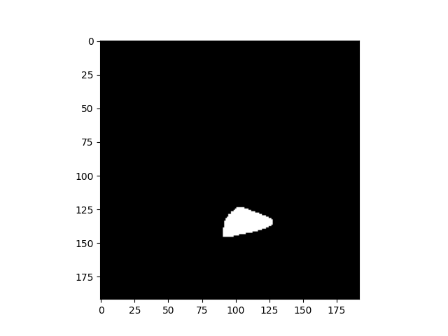
<matplotlib.image.AxesImage object at 0x751970eb9ad0>
However, we might be more interested in seeing how phosphene shape differs
for different electrodes.
For this we can use plot_argus_phosphenes() from
the viz module.
In addition to the data matrix, the function will also want an
ArgusII object implanted at the correct
location.
Consulting [Beyeler2019] tells us that the prosthesis was roughly implanted in the following location:
For now, let’s focus on the data from Subject 2:
data = fetch_beyeler2019(subjects='S2')
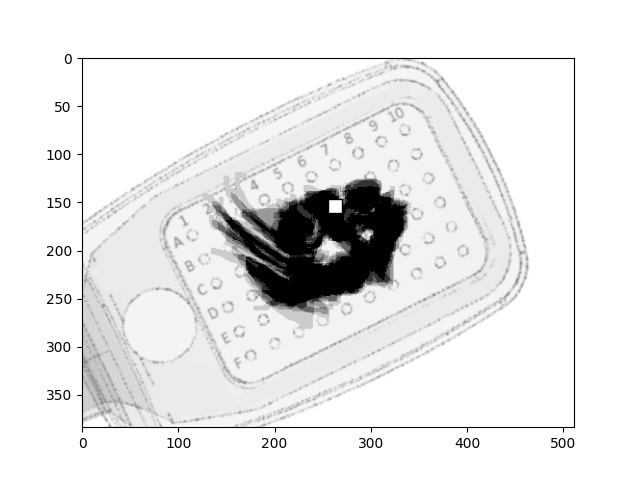
Passing both data and argus to
plot_argus_phosphenes() will then allow the
function to overlay the phosphene drawings over a schematic of the implant.
Here, phosphene drawings from different trials are averaged, and aligned with
the center of the electrode that was used to obtain the drawing:
from pulse2percept.viz import plot_argus_phosphenes
plot_argus_phosphenes(data, argus)

<Axes: >
Great! We have just reproduced a panel from Figure 2 in [Beyeler2019].
As [Beyeler2019] went on to show, the orientation of these phosphenes is well aligned with the map of nerve fiber bundles (NFBs) in each subject’s eye.
To see how the phosphene drawings line up with the NFBs, we can also pass an
AxonMapModel to the function.
Of course, we need to make sure that we use the correct dimensions. Subject
S2 had their optic disc center located 16.2 deg nasally, 1.38 deg superior
from the fovea:
from pulse2percept.models import AxonMapModel
model = AxonMapModel(loc_od=(16.2, 1.38))
plot_argus_phosphenes(data, argus, axon_map=model)
<Axes: >
Predicting phosphene shape
In addition, the AxonMapModel is well
suited to predict the shape of individual phosphenes. Using the values given
in [Beyeler2019], we can tailor the axon map parameters to Subject 2:
import numpy as np
model = AxonMapModel(rho=315, axlambda=500, loc_od=(16.2, 1.38),
                     xrange=(-30, 30), yrange=(-22.5, 22.5),
                     thresh_percept=1 / np.sqrt(np.e))
model.build()
AxonMapModel(ax_segments_range=(0, 50), axlambda=500,
             axon_pickle='axons.pickle',
             axons_range=(-180, 180), engine='cython',
             eye='RE', grid_type='rectangular',
             ignore_pickle=False, loc_od=(16.2, 1.38),
             min_ax_sensitivity=0.001, n_ax_segments=500,
             n_axons=1000, n_gray=None, n_jobs=1,
             n_threads=2, ndim=[2], noise=None, rho=315,
             scheduler='threading', spatial=AxonMapSpatial,
             temporal=None,
             thresh_percept=0.6065306597126334,
             verbose=True, vfmap=Watson2014Map(ndim=2),
             xrange=(-30, 30), xystep=0.25,
             yrange=(-22.5, 22.5))
Now we need to activate one electrode at a time, and predict the resulting
percept. We could build a Stimulus object
with a for loop that does just that, or we can use the following trick.
The stimulus’ data container is a (electrodes, timepoints) shaped 2D NumPy array. Activating one electrode at a time is therefore the same as an identity matrix whose size is equal to the number of electrodes. In code:
# Find the names of all the electrodes in the dataset:
electrodes = data.electrode.unique()
# Activate one electrode at a time:
import numpy as np
from pulse2percept.stimuli import Stimulus
argus.stim = Stimulus(np.eye(len(electrodes)), electrodes=electrodes)
Using the model’s
predict_percept(), we then get
a Percept object where each frame is the percept generated from activating
a single electrode:
Finally, we can visualize the ground-truth and simulated phosphenes side-by-side:
from pulse2percept.viz import plot_argus_simulated_phosphenes
fig, (ax_data, ax_sim) = plt.subplots(ncols=2, figsize=(15, 5))
plot_argus_phosphenes(data, argus, scale=0.75, ax=ax_data)
plot_argus_simulated_phosphenes(percepts, argus, scale=1.25, ax=ax_sim)
ax_data.set_title('Ground-truth phosphenes')
ax_sim.set_title('Simulated phosphenes')
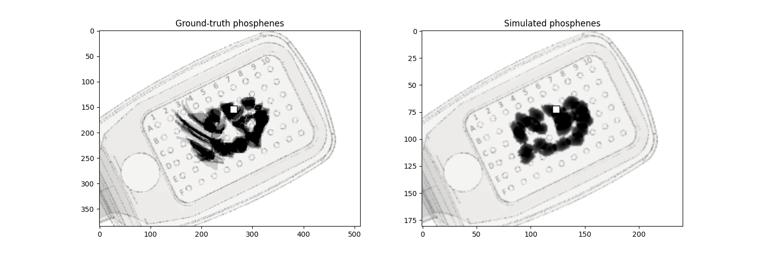
Text(0.5, 1.0, 'Simulated phosphenes')
Analyzing phosphene shape
The phosphene drawings also come annotated with different shape descriptors: area, orientation, and elongation. Elongation is also called eccentricity in the computer vision literature, which is not to be confused with retinal eccentricity. It is simply a number between 0 and 1, where 0 corresponds to a circle and 1 corresponds to an infinitesimally thin line (note that the Methods section of [Beyeler2019] got it wrong).
[Beyeler2019] made the point that if each phosphene could be considered a pixel (or essentially a blob), as is so often assumed in the literature, then most phosphenes should have zero elongation.
Instead, using Matplotlib’s histogram function, we can convince ourselves that most phosphenes are in fact elongated:
data = fetch_beyeler2019()
data.eccentricity.plot(kind='hist')
plt.xlabel('phosphene elongation')
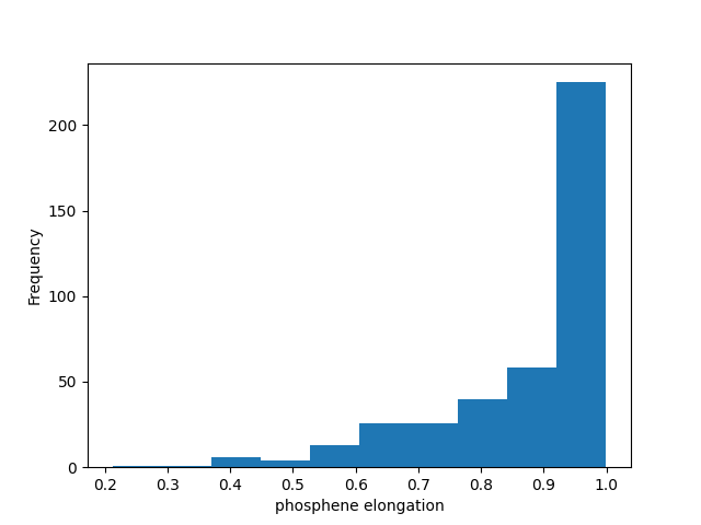
Text(0.5, 23.52222222222222, 'phosphene elongation')
Phosphenes are not pixels! And with that we have just reproduced Fig. 3C of [Beyeler2019].
Total running time of the script: (0 minutes 13.161 seconds)