Cortical implant gallery

pulse2percept supports the following cortical implants:

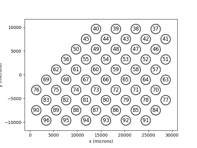
Orion Prosthesis System (Cortigent Inc.)

Orion contains 60 electrodes in a hex shaped grid inspired by Argus II.

import matplotlib.pyplot as plt
from pulse2percept.implants.cortex import *
import pulse2percept as p2p
import warnings
warnings.filterwarnings("ignore") # ignore matplotlib warnings

orion = Orion()
orion.plot(annotate=True)
plt.show()

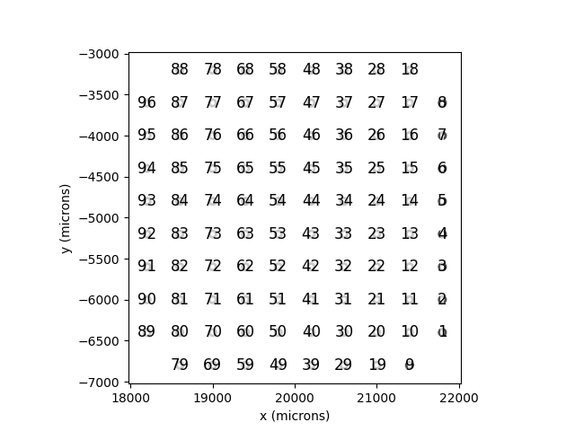
Cortivis Prosthesis System (Biomedical Technologies)

Cortivis is an implant with 96 electrodes in a square shaped grid.

cortivis = Cortivis()
cortivis.plot(annotate=True)
plt.show()

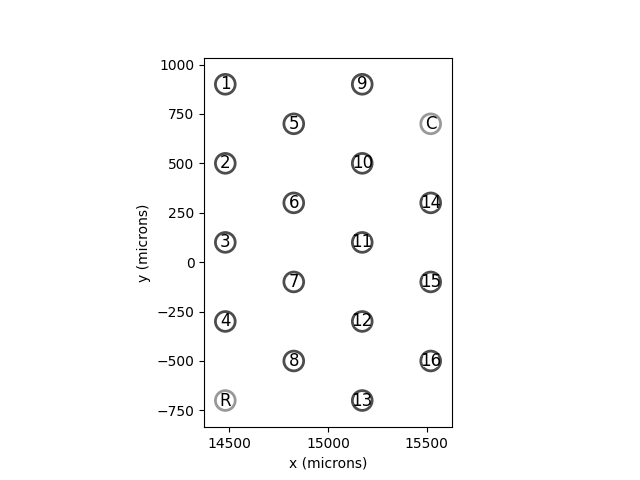
ICVP Prosthesis System (Sigenics Inc.)

ICVP is an implant with 16 primary electrodes in a hex shaped grid, along with 2 additional “reference” and “counter” electrodes.

icvp = ICVP()
icvp.plot(annotate=True)
plt.show()

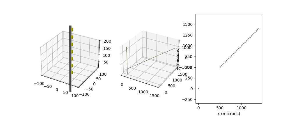
Neuralink Threads (Neuralink)

Neuralink is an implant consisting of one or more LinearEdgeThread, consisting of 32 electrodes.

These threads are designed to be 3D, and can be plotted in both 3D and 2D space, which will show the x-y projection of the points. Here are some examples showing the 1) a close up of the thread, 2) a 3D plot of two threads, and 3) the 2D projection of the two threads.

fig = plt.figure(figsize=(10, 4))
thread1 = LinearEdgeThread()
thread2 = LinearEdgeThread(500, 500, orient=[1, 1, 1])
ax0 = fig.add_subplot(131, projection='3d')
thread1.plot3D(ax=ax0)
ax0.set_xlim(-100, 100)
ax0.set_ylim(-100, 100)
ax0.set_zlim(10, 200)
ax1 = fig.add_subplot(132, projection='3d')
thread1.plot3D(ax=ax1)
thread2.plot3D(ax=ax1)
ax2 = fig.add_subplot(133)
thread1.plot(ax=ax2)
thread2.plot(ax=ax2)
plt.axis('equal')
plt.show()

Neuralink implants can be easily created from a NeuropythyMap enabling easy placement of implants across the cortical surface. See the neuropythy example for more details.

nmap = p2p.topography.NeuropythyMap(subject='fsaverage', regions=['v1'])
model = p2p.models.cortex.ScoreboardModel(rho=500, xrange=(-6, 0), yrange=(-5, 5), xystep=.25, vfmap=nmap).build()
nlink = Neuralink.from_neuropythy(nmap, xrange=model.xrange, yrange=model.yrange,
                                                      xystep=2, rand_insertion_angle=0)
print(len(nlink.implants), " total threads")
fig = plt.figure(figsize=(10, 4))
ax1 = fig.add_subplot(121, projection='3d')
model.plot3D(ax=ax1, style='cell')
nlink.plot3D(ax=ax1)
ax2 = fig.add_subplot(122)
model.plot(style='cell', ax=ax2)
nlink.plot(ax=ax2)

18  total threads
Warning: Plotting 2D projection of 3D data. You might want plot3D() instead

<Axes: xlabel='x (mm)', ylabel='y (mm)'>