Retinotopy: Predicting the perceptual effects of different visual field maps

Every computational model needs to assume a mapping between retinal and visual field coordinates. A number of these visual field maps are provided in the geometry module of the utilities subpackage:

• Curcio1990Map: The [Curcio1990] model simply assumes that one degree of visual angle (dva) is equal to 280 um on the retina.
• Watson2014Map: The [Watson2014] model extends [Curcio1990] by recognizing that the transformation between dva and retinal eccentricity is not linear (see Eq. A5 in [Watson2014]). However, within 40 degrees of eccentricity, the transform is virtually indistuingishable from [Curcio1990].
• Watson2014DisplaceMap: [Watson2014] also describes the retinal ganglion cell (RGC) density at different retinal eccentricities. In specific, there is a central retinal zone where RGC bodies are displaced centrifugally some distance from the inner segments of the cones to which they are connected through the bipolar cells, and thus from their receptive field (see Eq. 5 [Watson2014]).

All of these visual field maps follow the VisualFieldMap template. This means that they have to specify a dva2ret method, which transforms visual field coordinates into retinal coordinates, and a complementary ret2dva method.

Visual field maps

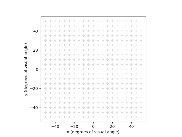
To appreciate the difference between the available visual field maps, let us look at a rectangular grid in visual field coordinates:

import pulse2percept as p2p
import matplotlib.pyplot as plt

grid = p2p.utils.Grid2D((-50, 50), (-50, 50), step=5)
grid.plot(style='scatter')
plt.xlabel('x (degrees of visual angle)')
plt.ylabel('y (degrees of visual angle)')
plt.axis('square')

Out:

(-55.0, 55.0, -55.0, 55.0)

Such a grid is typically created during a model’s build process and defines at which (x,y) locations the percept is to be evaluated.

However, these visual field coordinates are mapped onto different retinal coordinates under the three visual field maps:

transforms = [p2p.utils.Curcio1990Map,
              p2p.utils.Watson2014Map,
              p2p.utils.Watson2014DisplaceMap]
fig, axes = plt.subplots(ncols=3, sharey=True, figsize=(13, 4))
for ax, transform in zip(axes, transforms):
    grid.plot(transform=transform().dva2ret, style='cell', ax=ax)
    ax.set_title(transform().__class__.__name__)
    ax.set_xlabel('x (microns)')
    ax.set_ylabel('y (microns)')
    ax.axis('equal')

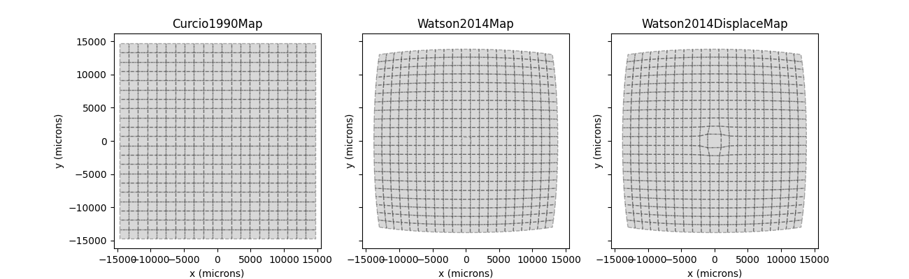
Whereas the [Curcio1990] map applies a simple scaling factor to the visual field coordinates, [Watson2014] uses a nonlinear transform. One thing to note is the RGC displacement zone in the third panel, which might lead to distortions in the fovea.

Perceptual distortions

The perceptual consequences of these visual field maps become apparent when used in combination with an implant.

For this purpose, let us create an AlphaAMS device on the fovea and feed it a suitable stimulus:

implant = p2p.implants.AlphaAMS(stim=p2p.stimuli.LogoUCSB())
implant.stim

Out:

Stimulus(data=[[0.], [0.], [0.], ..., [0.], [0.], [0.]],
         dt=0.001,
         electrodes=['A1' 'A2' 'A3' ... 'AN38' 'AN39' 'AN40'],
         is_charge_balanced=False, metadata=dict,
         shape=(1600, 1), time=None)

We can easily switch out the visual field maps by passing a retinotopy attribute to ScoreboardModel (by default, the scoreboard model will use [Curcio1990]):

fig, axes = plt.subplots(ncols=3, sharey=True, figsize=(13, 4))
for ax, transform in zip(axes, transforms):
    model = p2p.models.ScoreboardModel(xrange=(-6, 6), yrange=(-6, 6),
                                       retinotopy=transform())
    model.build()
    model.predict_percept(implant).plot(ax=ax)
    ax.set_title(transform().__class__.__name__)

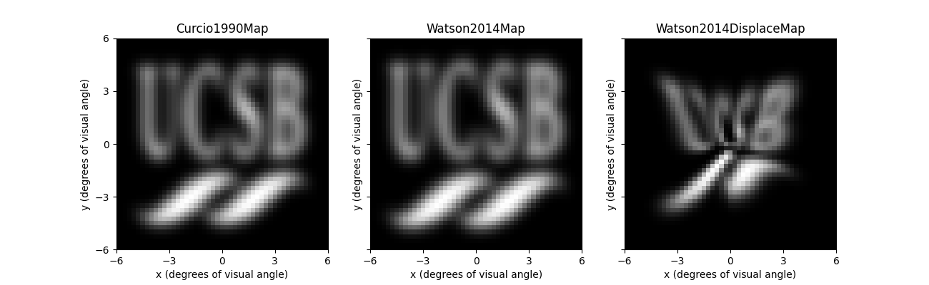
Whereas the left and center panel look virtually identical, the rightmost panel predicts a rather striking perceptual effect of the RGC displacement zone.

Creating your own visual field map

To create your own visual field map, you need to subclass the VisualFieldMap template and provide your own dva2ret and ret2dva methods. For example, the following class would (wrongly) assume that retinal coordinates are identical to visual field coordinates:

class MyVisualFieldMap(p2p.utils.VisualFieldMap):

    def dva2ret(self, xdva, ydva):
        return xdva, ydva

    def ret2dva(self, xret, yret):
        return xret, yret

To use it with a model, you need to pass retinotopy=MyVisualFieldMap() to the model’s constructor.