Beyeler et al. (2019): Focal percepts with the scoreboard model

This example shows how to apply the ScoreboardModel to a PRIMA75 implant.

The scoreboard model is a standard baseline model of retinal prosthesis stimulation, which assumes that electrical stimulation leads to the percept of focal dots of light, centered over the visual field location associated with the stimulated retinal field location \((x_{stim}, y_{stim})\), whose spatial intensity decays with a Gaussian profile [Hayes2003], [Thompson2003]:

\[I_{score}(x,y; \rho) = \exp \Big( -\frac{(x-x_{stim})^2 + (y-y_{stim})^2}{2 \rho^2} \Big)\]

where \(\rho\) is the spatial decay constant.

Important

As pointed out by [Beyeler2019], the scoreboard model does not well account for percepts generated by epiretinal implants, where incidental stimulation of retinal nerve fiber bundles leads to elongated, ‘streaky’ percepts.

In that case, use AxonMapModel instead.

The scoreboard model can be instantiated and run in three simple steps.

Creating the model

The first step is to instantiate the ScoreboardModel class by calling its constructor method.

The model simulates a patch of the visual field specified by xrange and yrange (in degrees of visual angle), sampled at a step size of xystep. The grid that is created from these parameters is equivalent to calling NumPy’s linspace(xrange[0], xrange[1], num=xystep).

By default, this patch is quite large, spanning 30deg x 30deg. Because PRIMA is rather small, we want to reduce the window size to 6deg x 6deg and sample it at 0.05deg resolution:

from pulse2percept.models import ScoreboardModel
model = ScoreboardModel(xrange=(-3, 3), yrange=(-3, 3), xystep=0.05)

Parameters you don’t specify will take on default values. You can inspect all current model parameters as follows:

print(model)

Out:

ScoreboardModel(engine=None, grid_type='rectangular',
                n_gray=None, n_jobs=1, n_threads=2,
                noise=None, retinotopy=Watson2014Map,
                rho=100, scheduler='threading',
                spatial=ScoreboardSpatial, temporal=None,
                thresh_percept=0, verbose=True,
                xrange=(-3, 3), xystep=0.05,
                yrange=(-3, 3))

This reveals a number of other parameters to set, such as:

• xrange, yrange: the extent of the visual field to be simulated, specified as a range of x and y coordinates (in degrees of visual angle, or dva). For example, we are currently sampling x values between -20 dva and +20dva, and y values between -15 dva and +15 dva.
• xystep: The resolution (in dva) at which to sample the visual field. For example, we are currently sampling at 0.25 dva in both x and y direction.
• thresh_percept: You can also define a brightness threshold, below which the predicted output brightness will be zero. It is currently set to 1/sqrt(e), because that will make the radius of the predicted percept equal to rho.

To change parameter values, either pass them directly to the constructor above or set them by hand, like this:

model.rho = 20

Then build the model. This is a necessary step before you can actually use the model to predict a percept, as it performs a number of expensive setup computations (e.g., building the spatial reference frame, calculating electric potentials):

model.build()

Out:

ScoreboardModel(engine=None, grid_type='rectangular',
                n_gray=None, n_jobs=1, n_threads=2,
                noise=None, retinotopy=Watson2014Map,
                rho=20, scheduler='threading',
                spatial=ScoreboardSpatial, temporal=None,
                thresh_percept=0, verbose=True,
                xrange=(-3, 3), xystep=0.05,
                yrange=(-3, 3))

Note

You need to build a model only once. After that, you can apply any number of stimuli – or even apply the model to different implants – without having to rebuild (which takes time).

Assigning a stimulus

The second step is to specify a visual prosthesis from the implants module.

In the following, we will create an PRIMA75 implant. By default, the implant will be centered over the fovea (at x=0, y=0) and aligned with the horizontal meridian (rot=0):

from pulse2percept.implants import PRIMA75
implant = PRIMA75()

We can visualize the implant and verify that we are simulating the correct patch of retina as follows:

model.plot()
implant.plot()

Out:

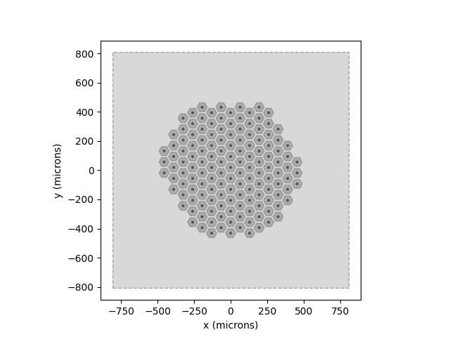
<AxesSubplot:xlabel='x (microns)', ylabel='y (microns)'>

The gray window indicates the extent of the grid that was created during model.build() using the values specified by xrange, yrange, and xystep. As we can see, the window well-covers the implant that we want to simulate.

The easiest way to assign a stimulus to the implant is to pass a NumPy array that specifies the current amplitude to be applied to every electrode in the implant.

For example, the following sends 10 microamps to all 142 electrodes of the implant:

import numpy as np
implant.stim = 10 * np.ones(142)

Note

Some models can handle stimuli that have both a spatial and a temporal component. The scoreboard model cannot.

Predicting the percept

The third step is to apply the model to predict the percept resulting from the specified stimulus. Note that this may take some time on your machine:

percept = model.predict_percept(implant)

Out:

/home/docs/checkouts/readthedocs.org/user_builds/pulse2percept/envs/stable/lib/python3.7/site-packages/pulse2percept/models/beyeler2019.py:94: UserWarning: Nonzero electrode-retina distances do not have any effect on the model output.
  warnings.warn(msg)

The resulting percept is stored in a Percept object, which is similar in organization to the Stimulus object: the data container is a 3D NumPy array (Y, X, T) with labeled axes xdva, ydva, and time.

The percept can be plotted as follows:

ax = percept.plot()
ax.set_title('Predicted percept')

Out:

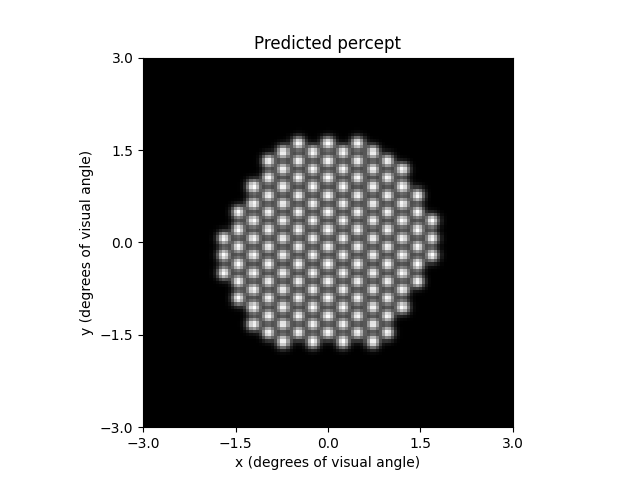
Text(0.5, 1.0, 'Predicted percept')

Note

Stimulation of the inferior retina leads to percepts appearing in the upper visual field. This is why the percept (with axes showing the visual field in degrees of visual angle) appears upside down with respect to the earlier figure of the implant (with axes showing retinal coordinates in microns).

By default, the plot method uses Matplotlib’s pcolor function. However, it can also be configured to use a hex grid (using Matplotlib’s hexbin function). Additional parameters can be passed to hexbin as keyword arguments of plot:

percept = model.predict_percept(implant)
percept.plot(kind='hex', cmap='inferno')

Out:

/home/docs/checkouts/readthedocs.org/user_builds/pulse2percept/envs/stable/lib/python3.7/site-packages/pulse2percept/models/beyeler2019.py:94: UserWarning: Nonzero electrode-retina distances do not have any effect on the model output.
  warnings.warn(msg)

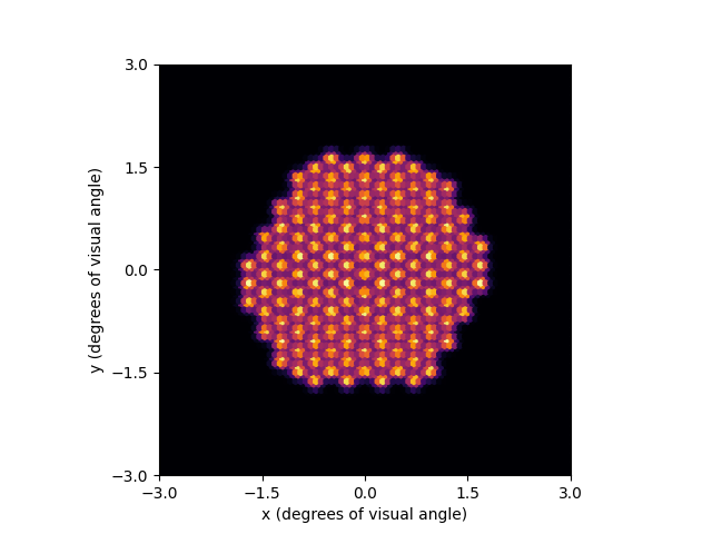
<AxesSubplot:xlabel='x (degrees of visual angle)', ylabel='y (degrees of visual angle)'>

Addressing individual electrodes

Alternatively, we can address an individual electrode. To show the electrode names, the implant can be plotted with annotate=True:

implant.plot(annotate=True)

Out:

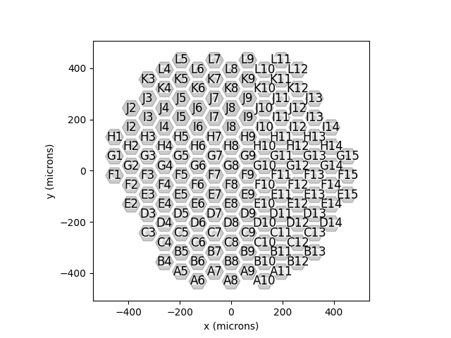
<AxesSubplot:xlabel='x (microns)', ylabel='y (microns)'>

This makes it easier to pick an electrode; e.g., F7:

implant.stim = {'F7': 10}

percept = model.predict_percept(implant)

percept.plot()

Out:

/home/docs/checkouts/readthedocs.org/user_builds/pulse2percept/envs/stable/lib/python3.7/site-packages/pulse2percept/models/beyeler2019.py:94: UserWarning: Nonzero electrode-retina distances do not have any effect on the model output.
  warnings.warn(msg)

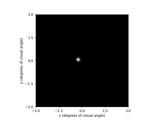
<AxesSubplot:xlabel='x (degrees of visual angle)', ylabel='y (degrees of visual angle)'>