Generating a stimulus from an image

This example shows how to use images as input stimuli for a retinal implant.

In addition to built-in stimuli such as BiphasicPulse and BiphasicPulseTrain, you can also load conventional images and convert them to stimuli using ImageStimulus.

Loading an image

An image can be loaded as follows:

stim = ImageStimulus('path-to-image.png')

By default, each pixel in the image is assigned to an electrode, and its grayscale value is encoded as an amplitude. If the image has more than 1 channel (e.g., RGB, RGBA), the image is flattened before each pixel/channel is assigned a different electrode. You can specify names for the electrodes, but the number of electrodes must match the number of pixels. By default, electrodes are labeled 1…N.

A number of images come pre-installed with pulse2percept, such as the logo of the Bionic Vision Lab (BVL) at UC Santa Barbara:

import pulse2percept as p2p
import numpy as np

logo = p2p.stimuli.LogoBVL()
print(logo)

Out:

LogoBVL(data=[[1.], [1.], [1.], ..., [1.], [1.], [0.]],
        dt=0.001, electrodes=<(1658880,) np.ndarray>,
        img_shape=(576, 720, 4), is_charge_balanced=False,
        metadata=dict, shape=(1658880, 1), time=None)

Inspecting the LogoBVL object, we can see that gray levels are converted to floats in the range [0, 1], and that the original 576x720x4 image is flattened so that each pixel can be assigned to an electrode.

We also notice that time=None, indicating that the stimulus does not have a time component. Thus we cannot apply temporal models to it.

LogoBVL can be assigned to a stimulus and used in conjunction with a phosphene model, just like any other Stimulus object.

Preprocessing an image

ImageStimulus objects come with a number of methods to process an image before it is passed to an implant. We can:

• invert the polarity of the image (applied to all channels except the alpha channel),
• convert RGB and RGBA images to grayscale using rgb2gray (note that a change in the number of pixels also means a change in the number of electrodes),
• resize the image to a new height x width (optionally using anti-aliasing),
• scale, shift, and rotate the image foreground (i.e., anything that’s not black),
• trim any black borders around the image.
• threshold the image using a number of commonly used techniques (e.g., Otsu’s method, adaptive thresholding, ISODATA),
• filter the image and extract edges (e.g., Sobel, Scharr, Canny, median filter),
• apply any input-output function not covered above (must accept an image as input and return another image of the same size).

Collectively, these methods should support arbitrarily complex image preprocessing strategies, including the ones commonly used by implants such as Argus II and Alpha-AMS.

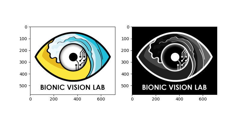
Let’s look at a concrete example. To get the BVL logo into proper shape, we need to convert the 4-channel RGBA image to grayscale. This can be done with rgb2gray. In addition, since grayscale values will be mapped to current ampltiudes, we may want to invert the image so that image edges appear bright on a dark background.

We can perform both actions in one line, and plot the result side-by-side with the original image:

logo_gray = logo.invert().rgb2gray()

import matplotlib.pyplot as plt
fig, (ax1, ax2) = plt.subplots(ncols=2, figsize=(8, 4))
logo.plot(ax=ax1)
logo_gray.plot(ax=ax2)

Out:

<AxesSubplot:>

As demonstrated above, multiple image processing steps can be performed in one line. This is possible because each method returns a copy of the processed image (without altering the original).

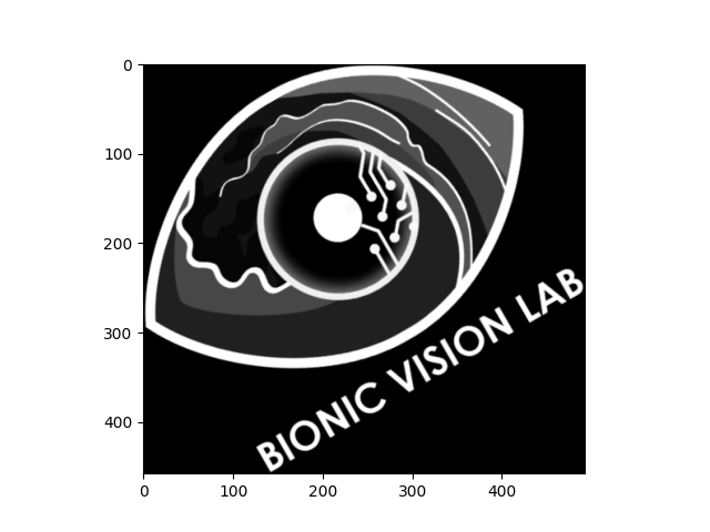
The following example takes the grayscale logo, shrinks it to 75% of its original size, rotates it by 30 degrees (counter-clockwise), and trims the black border around the image:

logo_gray.scale(0.75).rotate(30).trim().plot()

Out:

<AxesSubplot:>

As mentioned in the introduction above, the filter method provides a number of popular techniques to extract edges from the image, such as:

• 'sobel' to extract edges using the Sobel operator,
• 'scharr' to extract edges using the Scharr operator, and
• 'canny' to extract edges using the Canny algorithm.

Additional parameters (e.g., the standard deviation of the Gaussian filter for the Canny algorithm) can be passed as keyword arguments (e.g., filter('canny', sigma=3)).

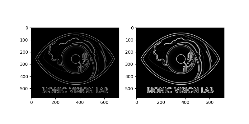
For example, we can use the Scharr operator as follows:

logo_edge = logo_gray.filter('scharr')

If more advanced image processing methods are required, we can use the apply method to apply literally any function to the image. The only requirement is that the function return an image of the same size.

For example, we can thicken the edges in the image by using a morphological operator (i.e., dilation) provided by scikit-image:

from skimage.morphology import dilation
logo_dilate = logo_edge.apply(dilation)

fig, (ax1, ax2) = plt.subplots(ncols=2, figsize=(8, 4))
# Edges extracted with the Scharr operator:
logo_edge.plot(ax=ax1)
# Edges thickened with dilation:
logo_dilate.plot(ax=ax2)

Out:

<AxesSubplot:>

We can also save the processed stimulus as an image:

logo_dilate.save('dilated_logo.png')

Using the image as input to a retinal implant

ImageStimulus can be used in combination with any ProsthesisSystem. We just have to resize the image first so that the number of pixels in the image matches the number of electrodes in the implant.

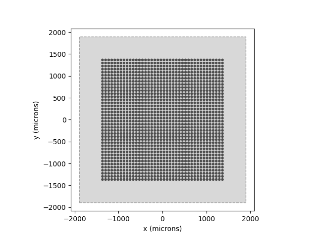
But let’s start from the top. The first two steps are to create a model and choose an implant:

# Simulate only what we need (14x14 deg sampled at 0.1 deg):
model = p2p.models.ScoreboardModel(xrange=(-7, 7), yrange=(-7, 7), xystep=0.1)
model.build()

from pulse2percept.implants import AlphaAMS
implant = AlphaAMS()

# Show the visual field we're simulating (dashed lines) atop the implant:
model.plot()
implant.plot()

Out:

<AxesSubplot:xlabel='x (microns)', ylabel='y (microns)'>

Since AlphaAMS is a 2D electrode grid, all we need to do is downscale the image to the size of the grid:

implant.stim = logo_gray.resize(implant.shape)

This way, the pixels of the image will be assigned to the electrodes in row-by-row order (i.e., we don’t need to specify the actual electrode names).

Note

If the implant is not a proper 2D grid, you will have to manually specify the input to each electrode.

In the near future, this will be done automatically using an implant’s preprocess method.

Then the implant can be passed to the model’s predict_percept method:

percept_gray = model.predict_percept(implant)

Note

Because neither ImageStimulus nor ScoreboardModel can handle time, the resulting percept will consist of a single image/frame.

To see what difference our image preprocessing makes on the quality of the resulting percept, we can re-run the model on logo_dilate and plot the two percepts side-by-side:

implant.stim = logo_dilate.trim().resize(implant.shape)
percept_dilate = model.predict_percept(implant)

fig, (ax1, ax2) = plt.subplots(ncols=2, figsize=(10, 4))
percept_gray.plot(ax=ax1)
percept_dilate.plot(ax=ax2)

Out:

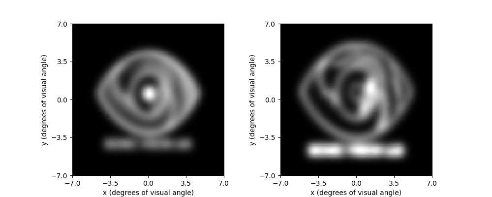
<AxesSubplot:xlabel='x (degrees of visual angle)', ylabel='y (degrees of visual angle)'>

Converting the image to a series of electrical pulses

ImageStimulus has an encode method to convert an image into a series of pulse trains (i.e., into electrical stimuli with a time component).

By default, the encode method will interpret the gray level of a pixel as the current amplitude of a BiphasicPulse with 0.46ms phase duration (500ms total stimulus duration). Gray levels in the range [0, 1] will be mapped onto currents in the range [0, 50] uA:

implant.stim = logo_dilate.trim().resize(implant.shape).encode()

We can customize the range of amplitudes to be used by passing a keyword argument; e.g. amp_range=(0, 20) to use currents in [0, 20] uA.

We can also specify our own pulse / pulse train to be used. First, we need to create the pulse we want to use (use amplitude 1 uA). Then, we need to pass it as an additional keyword argument; e.g., pulse=BiphasicPulseTrain(10, 1, 0.2, stim_dur=200) to use a 10Hz biphasic pulse train (0.2ms phase duration, overall duration 200 ms).

Using the image as input to a spatiotemporal model

Now, if we passed the new stimulus to ScoreboardModel, it would simply apply the model (in space) to every time point in the stimulus. To get a proper temporal response, we need to extend the scoreboard model with a proper temporal model, such as Horsager2009Temporal:

model = p2p.models.Model(spatial=p2p.models.ScoreboardSpatial,
                         temporal=p2p.models.Horsager2009Temporal)

Note

You can combine any spatial model (names ending in Spatial) with any temporal model (names ending in Temporal).

To make the model focus on the same visual field as above, we set xrange, yrange, and choose a proper xystep.

The rho parameter of the scoreboard model controls how much blur we get in the resulting percept. The value of this parameter should be set empirically to match the quality of the vision reported behaviorally by each implant user. For the purpose of this tutorial, we will set it to 50um:

model.build(xrange=(-7, 7), yrange=(-7, 7), xystep=0.1, rho=50)

Out:

Model(beta=3.43, dt=0.005, engine=None, eps=2.25,
      grid_type='rectangular', n_gray=None, n_jobs=1,
      n_threads=2, noise=None, retinotopy=Watson2014Map,
      rho=50, scheduler='threading',
      spatial=ScoreboardSpatial, tau1=0.42, tau2=45.25,
      tau3=26.25, temporal=Horsager2009Temporal,
      thresh_percept=0, verbose=True, xrange=(-7, 7),
      xystep=0.1, yrange=(-7, 7))

The predicted percept will now be a movie, where the spatial response (i.e., each frame of the movie) is primarily determined by the scoreboard model, but the temporal evolution of these frames is determined by the Horsager model.

By default, the model will output a movie frame every 20 ms (corresponding to a 50 Hz frame rate). The frame rate can be adjusted by passing a list of time points to predict_percept (e.g., t_percept=np.arange(500) to get an output every millisecond):

percept = model.predict_percept(implant)

The output of the model is a Percept object, which can be animated in IPython or Jupyter Notebook using the play method:

percept.play()

Once Loop Reflect

You can also save the percept as a movie:

percept.save('logo_percept.mp4')