Note
Click here to download the full example code
Threshold data from Horsager et al. (2009)
This example shows how to use the Horsager et al. (2009) dataset.
[Horsager2009] used a set of psychophysical detection tasks to determine perceptual thresholds in two Argus I users.
Important
You will need to install Pandas
(pip install pandas) for this dataset.
A typical task involved turning on a single electrode in the array and asking the subject if they saw something. If the subject did not detect a visual percept (i.e., a phosphene), the stimulus amplitude was increased. Using a staircase procedure, the researchers were able to determine the current amplitude at which subjects were able to detect a phosphene 50% of the time. This amplitude is called the threshold current, and it is stored in the “stim_amp” column of the dataset.
Note
Mean threshold currents were extracted from the main publication and its supplementary materials using Webplot Digitizer. Therefore, these data are provided without any guarantee of correctness or completeness.
Loading the dataset
The dataset can be loaded as a Pandas DataFrame:
from pulse2percept.datasets import load_horsager2009
data = load_horsager2009()
print(data)
Out:
    subject implant electrode  ... ref_interphase_dur  theta    source
0       S05  ArgusI        C3  ...                NaN  110.3     fig_3
1       S05  ArgusI        C3  ...                NaN  110.3     fig_3
2       S05  ArgusI        C3  ...                NaN  110.3     fig_3
3       S05  ArgusI        C3  ...                NaN  110.3     fig_3
4       S05  ArgusI        C3  ...                NaN  110.3     fig_3
..      ...     ...       ...  ...                ...    ...       ...
603     S06  ArgusI        D1  ...              0.075  147.0  fig_s3.2
604     S06  ArgusI        D1  ...              0.075  147.0  fig_s3.2
605     S06  ArgusI        D1  ...              0.075  147.0  fig_s3.2
606     S06  ArgusI        D1  ...              0.075  147.0  fig_s3.2
607     S06  ArgusI        D1  ...              0.075  147.0  fig_s3.2

[608 rows x 21 columns]
Inspecting the DataFrame tells us that there are 552 threshold measurements (the rows) each with 21 different attributes (the columns).
These attributes include specifiers such as “subject”, “electrode”, and “stim_type”. We can print all column names using:
data.columns
Out:
Index(['subject', 'implant', 'electrode', 'task', 'stim_type', 'stim_dur',
       'stim_freq', 'stim_amp', 'pulse_type', 'pulse_dur', 'pulse_num',
       'interphase_dur', 'delay_dur', 'ref_stim_type', 'ref_freq', 'ref_amp',
       'ref_amp_factor', 'ref_pulse_dur', 'ref_interphase_dur', 'theta',
       'source'],
      dtype='object')
Note
The meaning of all column names is explained in the docstring of
the load_horsager2009 function.
For example, “stim_type” corresponds to the different stimulus types that were used in the paper:
data.stim_type.unique()
Out:
array(['single_pulse', 'fixed_duration', 'variable_duration',
       'fixed_duration_supra', 'bursting_triplets',
       'bursting_triplets_supra', 'latent_addition'], dtype=object)
The first entry, “single_pulse”, corresponds to the single biphasic pulse used to produce Figure 3. We can verify which figure a data point came from by inspecting the “source” column.
To select all the “single_pulse” rows, we can index into the DataFrame as follows:
print(data[data.stim_type == 'single_pulse'])
Out:
   subject implant electrode  ... ref_interphase_dur  theta    source
0      S05  ArgusI        C3  ...                NaN  110.3     fig_3
1      S05  ArgusI        C3  ...                NaN  110.3     fig_3
2      S05  ArgusI        C3  ...                NaN  110.3     fig_3
3      S05  ArgusI        C3  ...                NaN  110.3     fig_3
4      S05  ArgusI        C3  ...                NaN  110.3     fig_3
..     ...     ...       ...  ...                ...    ...       ...
75     S06  ArgusI        D1  ...                NaN  132.0  fig_s3.1
76     S06  ArgusI        D1  ...                NaN  132.0  fig_s3.1
77     S06  ArgusI        D1  ...                NaN  132.0  fig_s3.1
78     S06  ArgusI        D1  ...                NaN  132.0  fig_s3.1
79     S06  ArgusI        D1  ...                NaN  132.0  fig_s3.1

[80 rows x 21 columns]
This leaves us with 80 rows, some of which come from Figure 3, others from Figure S3.1 in the supplementary material.
An alternative to indexing into the DataFrame is to load only a subset of the data:
print(load_horsager2009(stim_types='single_pulse'))
Out:
   subject implant electrode  ... ref_interphase_dur  theta    source
0      S05  ArgusI        C3  ...                NaN  110.3     fig_3
1      S05  ArgusI        C3  ...                NaN  110.3     fig_3
2      S05  ArgusI        C3  ...                NaN  110.3     fig_3
3      S05  ArgusI        C3  ...                NaN  110.3     fig_3
4      S05  ArgusI        C3  ...                NaN  110.3     fig_3
..     ...     ...       ...  ...                ...    ...       ...
75     S06  ArgusI        D1  ...                NaN  132.0  fig_s3.1
76     S06  ArgusI        D1  ...                NaN  132.0  fig_s3.1
77     S06  ArgusI        D1  ...                NaN  132.0  fig_s3.1
78     S06  ArgusI        D1  ...                NaN  132.0  fig_s3.1
79     S06  ArgusI        D1  ...                NaN  132.0  fig_s3.1

[80 rows x 21 columns]
Plotting the data
Arguably the most important column is “stim_amp”. This is the current amplitude of the different stimuli (single pulse, pulse trains, etc.) used at threshold.
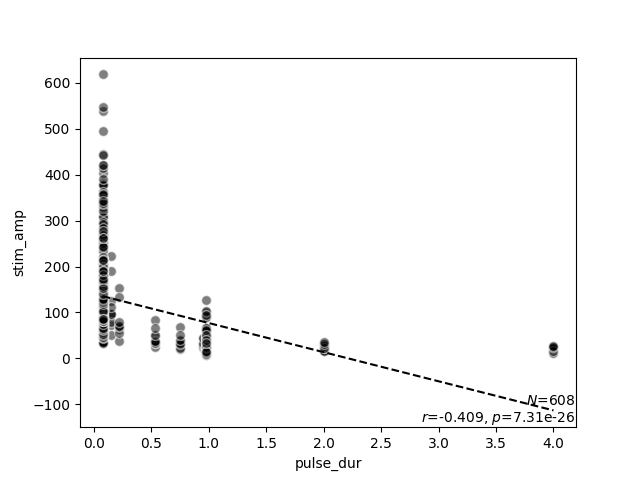
We might be interested in seeing how threshold amplitude varies as a function of pulse duration. We could either use Matplotlib to generate a scatter plot or use pulse2percept’s own visualization function:
from pulse2percept.viz import scatter_correlation
scatter_correlation(data.pulse_dur, data.stim_amp)
Out:
<AxesSubplot:xlabel='pulse_dur', ylabel='stim_amp'>
scatter_correlation above generates a scatter
plot of the stimulus amplitude as a function of pulse duration, and performs
linear regression to calculate a correlation $r$ and a $p$ value.
As expected from the literature, now it becomes evident that stimulus
amplitude is negatively correlated with pulse duration (no matter the exact
stimulus used).
Recreating the stimuli
To recreate the stimulus used to obtain a specific data point, we need to use the values specified in the different columns of a particular row.
For example, the first row of the dataset specifies the stimulus used to obtain the threshold current for subject S05 on Electrode C3 using a single biphasic pulse:
row = data.loc[0, :]
print(row)
Out:
subject                          S05
implant                       ArgusI
electrode                         C3
task                       threshold
stim_type               single_pulse
stim_dur                         200
stim_freq                        NaN
stim_amp                     179.793
pulse_type            cathodic_first
pulse_dur                      0.075
pulse_num                          1
interphase_dur                 0.075
delay_dur                        NaN
ref_stim_type                    NaN
ref_freq                         NaN
ref_amp                          NaN
ref_amp_factor                   NaN
ref_pulse_dur                    NaN
ref_interphase_dur               NaN
theta                          110.3
source                         fig_3
Name: 0, dtype: object
Using BiphasicPulse, we can create the
pulse to specifications:
from pulse2percept.stimuli import BiphasicPulse
stim = BiphasicPulse(row['stim_amp'], row['pulse_dur'],
                     interphase_dur=row['interphase_dur'],
                     stim_dur=row['stim_dur'], electrode=row['electrode'])
We can zoom in on the first 10 ms to see the stimulus waveform:
import numpy as np
stim.plot(time=np.arange(0, 10, 0.01))
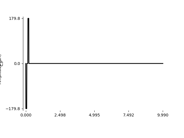
Out:
<AxesSubplot:ylabel='C3'>
Total running time of the script: ( 0 minutes 0.284 seconds)